Archive
Predicting the size of the Linux kernel binary
How big is the binary for the Linux kernel? Depending on the value of around 15,000 configuration options, the size of the version 5.8 binary could be anywhere between 7.3Mb and 2,134 Mb.
Who is interested in the size of the Linux kernel binary?
We are not in the early 1980s, when memory for a desktop microcomputer often topped out at 64K, and software was distributed on 360K floppies (720K when double density arrived; my companies first product was a code optimizer which reduced program size by around 10%).
While desktop systems usually have oodles of memory (disk and RAM), developers targeting embedded systems seek to reduce costs by minimizing storage requirements, security conscious organizations want to minimise the attack surface of the programs they run, and performance critical systems might want a kernel that fits within a processors’ L2/L3 cache.
When management want to maximise the functionality supported by a kernel within given hardware resource constraints, somebody gets the job of building kernels supporting various functionality to find out the size of the binaries.
At around 4+ minutes per kernel build, it’s going to take a lot of time (or cloud costs) to compare lots of options.
The paper Transfer Learning Across Variants and Versions: The Case of Linux Kernel Size by Martin, Acher, Pereira, Lesoil, Jézéquel, and Khelladi describes an attempt to build a predictive model for the size of the kernel binary. This paper includes an extensive list of references.
The author’s approach was to first obtain lots of kernel binary sizes by building lots of kernels using random permutations of on/off options (only on/off options were changed). Seven kernel versions between 4.13 and 5.8 were used, producing 243,323 size/option setting combinations (complete dataset). This data was used to train a machine learning model.
The accuracy of the predictions made by models trained on a single kernel version were accurate within that kernel version, but the accuracy of single version trained models dropped dramatically when used to predict the binary size of later kernel versions, e.g., a model trained on 4.13 had an accuracy of 5% MAPE predicting 4.13, when predicting 4.15 the accuracy is 20%, and 32% accurate predicting 5.7.
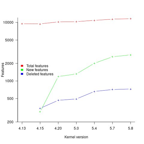
I think that the authors’ attempt to use this data to build a model that is accurate across versions is doomed to failure. The rate of change of kernel features (whose conditional compilation is supported by one or more build options) supported by Linux is too high to be accurately modelled based purely on information of past binary sizes/options. The plot below shows the total number of features, newly added, and deleted features in the modelled version of the kernel (code+data):
What is the range of impacts of each build option, on binary size?
If each build option is independent of the others (around 44% of conditional compilation directives in the kernel source contain one option), then the fitted coefficients of a simple regression model gives the build size increment when the corresponding option is enabled. After several cpu hours, the 92,562 builds involving 9,469 options in the version 4.13 build data were fitted. The plot below shows a sorted list of the size contribution of each option; the model  is 0.72, i.e., quite a good fit (code+data):

While the mean size increment for an enabled option is 75K, around 40% of enabled options decreases the size of the kernel binary. Modelling pairs of options (around 38% of conditional compilation directives in the kernel source contain two options) will have some impact on the pattern of behavior seen in the plot, but given the quality of the current model ( is 0.72) the change is unlikely to be dramatic. However, the simplistic approach of regression fitting the 90 million pairs of option interactions is not practical.
What might be a practical way of estimating binary size for any kernel version?
The size of a binary is essentially the quantity of code+static data it contains.
An estimate of the quantity of conditionally compiled source code dependent on a given option is likely to be a good proxy for that option’s incremental impact on binary size.
It’s trivial to scan source code for occurrences of options in conditional compilation directives, and with a bit more work, the number of lines controlled by the directive can be counted.
There has been a lot of evidence-based research on software product lines, and feature macros in particular. I was expecting to find a dataset listing the amount of code controlled by build options in Linux, but the data I can find does not measure Linux.
The Martin et al. build data is perfectfor creating a model linking quantity of conditionally compiled source code to change of binary size.
Multi-state survival modeling of a Jira issues snapshot
Work items in a formal development process progress through a series of stages, e.g., starting at Open, perhaps moving to Withdrawn or Merged with another item, eventually reaching Development, and finishing at Done (with a few being Reopened, i.e., moving back to the start of the process).
This process can be modelled as a Markov chain, provided data on each stage of the process is available, for each work item; allowing values such as average time spent in each state and transition probabilities to be calculated.
The Jira issue/task/bug/etc tracking system has an option to generate a snapshot of the current status of work items in the system. The snapshot information on each item includes: start-date, current-state, time-in-state, date-of-snapshot.
If we assume that all work items pass through the same sequence of states, from Open to Done, then the snapshot contains enough information to build a multi-state survival model.
The key information is time-in-state, which can be used to calculate the date/time when an item transitioned from its previous state to its current state, providing a required link between all states.
How is a multi-state survival model better than creating a distinct survival model for each state?
The calculation of each state in a multi-state model takes into account information from the succeeding state, i.e., the time-in-state value in the succeeding state provides timing (from the Start state) on when a work item transitioned from its previous state. While this information could be added to each of the distinct models, it’s simpler to bundle everything together in one model.
A data analysis article by Robert Krasinski linked to the data used 🙂 The data does not include a description of the columns, but most of the names appear self-explanatory (I have no idea what key might be). Each of the 3,761 rows includes a story-point estimate, team-id, and a tag name for the work item.
Building a multi-state model provides a means for estimating the impact of team-id and story-points on time-in-state. I would expect items with higher story-point estimates to spend longer in Development, but I’m not sure how much difference there will be on other states.
I pruned the 22 states present in the data down to the following sequence of 13. Items might be Withdrawn or Merged with others items at any time, but I’m keeping things simple. These two states should also be absorbing in that there is no exit from them, I faked this by adding a transition to Done.
           Open
           Withdrawn
           Merged
           Backlog
           In Analysis
           In Refinement
           Ready for Development
           In Development
           Code Review
           Ready for Test
           In Testing
           Ready for Signoff
Done |
I’m familiar with building survival models, but have only ever built a couple of multi-state survival models. R supports several packages, which is the best one to use for this minimalist multi-state dataset?
The msm package is very much into state transition probabilities, or at least that is the impression I got from reading its manual. flexsurv and mstate are other packages I looked at. I decided to stay with the survival package, the default for simpler problems; the manuals contained lots of examples and some of them appeared similar to my problem.
Each row of work item information in the Jira snapshot looks something like the following:
X daysInStatus start status obsdate 1 0.53 2020-05-12 In Development 2020-05-18 |
This work item transitioned from state Ready for Development at time  to state In Development at time
  , and was still in state In Development at time
  (when the snapshot was taken); the
  is a small interval used to separate the states.
As is often the case with R packages, most of the work went into figuring out how to call the library functions with the data formatted just so, plus of course my own misunderstandings. Once the data was cleaned and process, the analysis was one line of code plus one to print the results; for instance, to estimate the mean time in each state by story-point value (code+data):
sp_fit=survfit(Surv(tstop-tstart, state) ~ sp, data=merged_status) print(sp_fit) |
Given the uncertainties in this model building process, I’m not going to discuss the results. This post is a proof of concept, which others can apply when the sequence of states is known with some degree of confidence, and good reasons for noise in the data are available.
Including natural language text topics in a regression model
The implementation records for a project sometimes include a brief description of each task implemented. There will be some degree of similarity between the implementation of some tasks. Is it possible to calculate the degree of similarity between tasks from the text in the task descriptions?
Over the years, various approaches to measuring document similarity have been proposed (more than you probably want to know about natural language processing).
One of the oldest, simplest and widely used technique is term frequency–inverse document frequency (tf-idf), which is based on counting word frequencies, i.e., is word context is ignored. This technique can work well when there are a sufficient number of words to ensure a good enough overlap between similar documents.
When the description consists of a sentence or two (i.e., a summary), the problem becomes one of sentence similarity, not document similarity (so tf-idf is unlikely to be of any use).
Word context, in a sentence, underpins the word embedding approach, which represents a word by an n-dimensional vector calculated from the local sentence context in which the word occurs (derived from a large amount of text). Words that are closer, in this vector space, are expected to have similar meanings. One technique for calculating the similarity between sentences is to compare the averages of the word embedding of the words they contain. However, care is needed; words appearing in the same context can create sentences having different meanings, as in the following (calculated sentence similarity in the comments):
import spacy nlp=spacy.load("en_core_web_md") # _md model needed for word vectors nlp("the screen is black").similarity(nlp("the screen is white")) # 0.9768339369182919 # closer to 1 the more similar the sentences nlp("implementing widgets would be little effort").similarity(nlp("implementing widgets would be a huge effort")) # 0.9636533803238744 nlp("the screen is black").similarity(nlp("implementing widgets would be a huge effort")) # 0.6596892830922606 |
The first pair of sentences are similar in that they are about the characteristics of an object (i.e., its colour), while the second pair are similar in that are about the quantity of something (i.e., implementation effort), and the third pair are not that similar.
The words in a document, or summary, are about some collection of topics. A set of related documents are likely to contain a discussion of a set of related topics in varying degrees. Latent Dirichlet allocation (LDA) is a widely used technique for calculating a set of (unseen) topics from a set of documents and their contained words.
A recent paper attempted to estimate task effort based on the similarity of the task descriptions (using tf-idf). My last semi-serious attempt to extract useful information from text, some years ago, was a miserable failure (it’s a very hard problem). Perhaps better techniques and tools are now available for me to leverage (my interest is in understanding what is going on, not making predictions).
My initial idea was to extract topics from task data, and then try to add these to regression models of task effort estimation, to see what impact they had. Searching to find out what researchers have recently been doing in this area, I was pleased to see that others were ahead of me, and had implemented R packages to do the heavy lifting, in particular:
- The
stmpackage supports the creation of Structural Topic Models; these add support for covariates to influence the process of fitting LDA models, i.e., a correlation between the topics and other variables in the data. Uses of STM appear to be oriented towards teasing out differences in topics associated with different values of some variable (e.g., political party), and the package authors have written papers analysing political data. - The
psychtmpackage supports what the authors call supervised latent Dirichlet allocation with covariates (SLDAX). This handles all the details needed to include the extracted LDA topics in a regression model; exactly what I was after. The user interface and documentation for this package is not as polished as thestmpackage, but the code held together as I fumbled my way through.
To experiment using these two packages I used the SiP dataset, which includes summary text for each task, and I have previously analysed the estimation task data.
The stm package:
The textProcessor function handles all the details of converting a vector of strings (e.g., summary text) to internal form (i.e., handling conversion to lower case, removing stop words, stemming, etc).
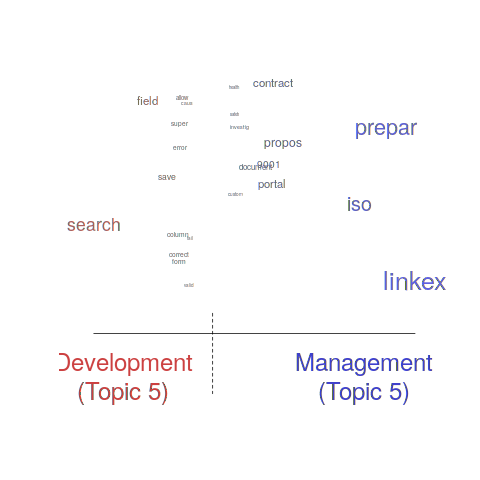
One of the input variables to the LDA process is the number of topics to use. Picking this value is something of a black art, and various functions are available for calculating and displaying concepts such as topic semantic coherence and exclusivity, the most commonly used words associated with a topic, and the documents in which these topics occur. Deciding the extent to which 10 or 15 topics produced the best results (values that sounded like a good idea to me) required domain knowledge that I did not have. The plot below shows the extent to which the words in topic 5 were associated with the Category column having the value “Development” or “Management” (code+data):
The psychtm package:
The prep_docs function is not as polished as the equivalent stm function, but the package’s first release was just last year.
After the data has been prepared, the call to fit a regression model that includes the LDA extracted topics is straightforward:
sip_topic_mod=gibbs_sldax(log(HoursActual) ~ log(HoursEstimate), data = cl_info,
                         docs = docs_vocab$documents, model = "sldax",
K = 10 # number of topics) |
where: log(HoursActual) ~ log(HoursEstimate) is the simplest model fitted in the original analysis.
The fitted model had the form:  , with the calculated coefficient for some topics not being significant. The value
  is close to that fitted in the original model. The value of
  is the fraction of the calculated to be present in the Summary text of the corresponding task.
I’m please to see that a regression model can be improved by adding topics derived from the Summary text.
The SiP data includes other information such as work Category (e.g., development, management), ProjectCode and DeveloperId. It is to be expected that these factors will have some impact on the words appearing in a task Summary, and hence the topics (the stm analysis showed this effect for Category).
When the model formula is changed to: log(HoursActual) ~ log(HoursEstimate)+ProjectCode, the quality of fit for most topics became very poor. Is this because ProjectCode and topics conveyed very similar information, or did I need to be more sophisticated when extracting topic models? This needs further investigation.
Can topic models be used to build prediction models?
Summary text can only be used to make predictions if it is available before the event being predicted, e.g., available before a task is completed and the actual effort is known. My interest in model building is to understand the processes involved, so I am not worried about when the text was created.
My own habit is to update, or even create Summary text once a task is complete. I asked Stephen Cullen, my co-author on the original analysis and author of many of the Summary texts, about the process of creating the SiP Summary sentences. His reply was that the Summary field was an active document that was updated over time. I suspect the same is true for many task descriptions.
Not all estimation data includes as much information as the SiP dataset. If Summary text is one of the few pieces of information available, it may be possible to use it as a proxy for missing columns.
Perhaps it is possible to extract information from the SiP Summary text that is not also contained in the other recorded information. Having been successful this far, I will continue to investigate.
Another nail for the coffin of past effort estimation research
Programs are built from lines of code written by programmers. Lines of code played a starring role in many early effort estimation techniques (section 5.3.1 of my book). Why would anybody think that it was even possible to accurately estimate the number of lines of code needed to implement a library/program, let alone use it for estimating effort?
Until recently, say up to the early 1990s, there were lots of different computer systems, some with multiple (incompatible’ish) operating systems, almost non-existent selection of non-vendor supplied libraries/packages, and programs providing more-or-less the same functionality were written more-or-less from scratch by different people/teams. People knew people who had done it before, or even done it before themselves, so information on lines of code was available.
The numeric values for the parameters appearing in models were obtained by fitting data on recorded effort and lines needed to implement various programs (63 sets of values, one for each of the 63 programs in the case of COCOMO).
How accurate is estimated lines of code likely to be (this estimate will be plugged into a model fitted using actual lines of code)?
I’m not asking about the accuracy of effort estimates calculated using techniques based on lines of code; studies repeatedly show very poor accuracy.
There is data showing that different people implement the same functionality with programs containing a wide range of number of lines of code, e.g., the 3n+1 problem.
I recently discovered, tucked away in a dataset I had previously analyzed, developer estimates of the number of lines of code they expected to add/modify/delete to implement some functionality, along with the actuals.
The following plot shows estimated added+modified lines of code against actual, for 2,692 tasks. The fitted regression line, in red, is:  (the standard error on the exponent is
  ), the green line shows
  (code+data):
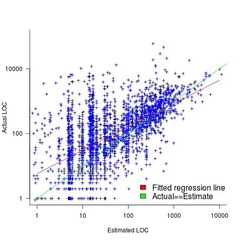
The fitted red line, for lines of code, shows the pattern commonly seen with effort estimation, i.e., underestimating small values and over estimating large values; but there is a much wider spread of actuals, and the cross-over point is much further up (if estimates below 50-lines are excluded, the exponent increases to 0.92, and the intercept decreases to 2, and the line shifts a bit.). The vertical river of actuals either side of the 10-LOC estimate looks very odd (estimating such small values happen when people estimate everything).
My article pointing out that software effort estimation is mostly fake research has been widely read (it appears in the first three results returned by a Google search on software fake research). The early researchers did some real research to build these models, but later researchers have been blindly following the early ‘prophets’ (i.e., later research is fake).
Lines of code probably does have an impact on effort, but estimating lines of code is a fool’s errand, and plugging estimates into models built from actuals is just crazy.
COCOMO: Not worth serious attention
The Constructive Cost Model (COCOMO) was introduced to the world by the book “Software Engineering Economics” by Barry Boehm; this particular version of the model is now known by the year of publication, COCOMO 81. The book describes a model that estimates software project cost drivers, such as effort (in man months) and elapsed time; the data from the 63 projects used to help calibrate the equations appears on pages 496-497.
Only having 63 measurements to model such a complex problem means any predictions will have very wide error bounds; however, the small amount of data did not stop Boehm building an academic career out of over-fitting these 63 measurements using 17 input parameters (the COCOMO II book came out in 2000 and was initially calibrated by fitting 22 parameters to 83 measurement points and then by fitting 23 parameters to 161 measurement points; the measurement data does not appear to be publicly available).
A sentence on page 493 suggests that over-fitting may not be the only problem to be found in the data analysis: “The calibration and evaluation of COCOMO has not relied heavily on advanced statistical techniques.”
Let’s take the original data and duplicate the original analysis, before trying something more advanced (code+data).
A central plank of the COCOMO model is the equation:  , where
  is total effort in man months,
  a constant obtained by fitting the data,
  thousands of lines of source code and
  a constant obtained by fitting the data.
This post discusses fitting this equation for the three modes of software projects defined by Boehm (along with the equations he fitted):
- Organic, relatively small teams operating in a highly familiar environment:
 ,
, - Embedded, the product has to operate within strongly coupled, complex, hardware, software and operational procedures such as air traffic control:
 ,
, - Semidetached, an intermediate stage between the two extremes:
 .
.
The plot below shows kSLOC against Effort, with solid lines fitted using what I guess was Boehm’s approach and dashed lines showing fitted lines after removing outliers (Figure 6-5 in the book has the x/y axis switched; the points in the above plot appear to match those in this figure):
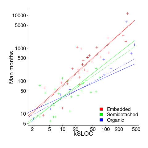
The fitted equations are (the standard error on the multiplier, , is around ±30%, while on the exponent, , the absolute value varies between ±0.1 and ±0.2):
- Organic:
 , after outlier removal
- Embedded:
 , after outlier removal
- Semidetached:
 , after outlier removal
  .
.
The only big difference is for Organic, which is very different. My first reaction on seeing this was to double check the values used against those in the book. How did Boehm make such a big mistake and why has nobody spotted it (or at least said anything) before now? Papers by Boehm’s students do use fancy statistical techniques and contain lots of tables of numbers relating to COCOMO 81, but no mention of what model they actually found to be a good fit.
The table on pages 496-497 contains man month estimates made using Boehm’s equations (the EST column). The values listed are a close match to the values I calculated using Boehm’s Semidetached equation, but there are many large discrepancies between printed values and values I calculated (using Boehm’s equations) for Organic and Embedded. If the data in this table contains a lot of mistakes, it may explain why I get very different values fitting the data for Organic. Some ther columns contain values calculated using the listed EST values and the few I have checked are correct, so if there was an error in the EST value calculation it must have occurred early in the chain of calculations.
The data for each of the three modes of software development contain several in your face outliers (assuming the values are correct). Based on the fitted equations is does not look like Boehm removed these (perhaps detecting outliers is an advanced technique).
Once the very obvious outliers are removed the quadratic equation,  , becomes a viable competing model. Unfortunately we don’t have enough data to do a serious comparison of this equation against the COCOMO equation.
In practice the COCOMO 81 model has been found to be highly inaccurate and very much dependent upon the interpretation of the input parameters.
Further down on page 493 we have: “I have become convinced that the software field is currently too primitive, and cost driver interaction too complex, for standard statistical techniques to make much headway;”.
With so much complexity and uncertainty, careful application of statistical techniques is the only way of reliable way of distinguishing any signal from noise.
COCOMO does not deserve anymore serious attention (the code+data includes some attempts to build alternative models, before I decided it was not worth the effort).
Data cleaning: The next step in empirical software engineering
Over the last 10 years software engineering researchers have gone from a state of data famine to being deluged with data. Until recently these researchers have been acting like children at a birthday party, rushing around unwrapping all the presents to see what is inside and quickly moving onto the next one. A good example of this are those papers purporting to have found a power law relationship between two constructs by simply plotting the data using log axis and drawing a straight line through the data; hey look, a power law, isn’t that interesting? Hopefully, these days, reviewers are starting to wise up and insist that any claims of a power law be checked.
Data cleaning is a very important topic that unfortunately appears to be missing from many researchers’ approach to data analysis. The quality of a model built from data is only as good as the quality of the data used to build it. Anybody who is interested in building models that connect to the real world of software engineering, rather than just getting another paper published, has to consider the messiness that gets added to data by the software developers who are intimately involved in the processes that generated the artifacts (e.g., source code, bug reports).
I have jut been reading a paper containing some unsettling numbers (It’s not a Bug, it’s a Feature: On the Data Quality of Bug Databases). A manual classification of over 7,000 issues reported against various large Java applications found that 42.6% of the issues were misclassified (e.g., a fault report was actually a request for enhancement), resulting in a change of status of 39% of the files once thought to contain a fault to not actually containing a fault (any fault prediction models built assuming the data in the fault database was correct now belong in the waste bin).
What really caught my eye about this research was the 725 hours (90 working days) invested by the researchers doing the manual classification (one person + independent checking by another). Anybody can extracts counts of this that and the other from the many repositories now freely available, generate fancy looking plots from them and add in some technobabble to create a paper. Real researchers invest lots of their time figuring out what is really going on.
These numbers are a wakeup call for all software engineering researchers. The data you are using needs to be thoroughly checked and be prepared to invest a lot of time doing it.
Preferential attachment applied to frequency of accessing a variable
If, when writing code for a function, up to the current point in the code  distinct local variables have been accessed for reading
  times (
 ), will the next read access be from a previously unread local variable and if not what is the likelihood of choosing each of the distinct variables (global variables are ignored in this analysis)?
Short answer:
- With probability
 select a new variable to access,
 - otherwise select a variable that has previously been accessed in the function, with the probability of selecting a particular variable being proportional to
 (where
  is the number of times the variable has previously been read from.
The longer answer is below as another draft section from my book Empirical software engineering with R. As always comments and pointers to more data welcome. R code and data here.
The discussion on preferential attachment is embedded in a discussion of model building.
What kind of model to build?
The obvious answer to the question of what kind of model to build is, the cheapest one that produces the desired output.
Many of the model building techniques discussed in this book find patterns in the data and effectively return one or more equations that produce output similar to the data given some set of inputs; the equations are the model.
The advantage of this approach is that in many cases the implementation of the model building has been automated (I don’t say much about those that have not yet been automated), the user contribution is in choosing which kind of model to build. In some cases the R function requires that the user provide a general direction of attack (e.g., the form of function to use in fitting a nonlinear regression).
An alternative kind of model is one whose output is obtained by running an iterative algorithm, e.g., a time series created by calculating the next value in a sequence from one or more previous values.
In most cases a great deal of domain knowledge is required of the user building the model, while in a few cases an automated procedure for creating the iterative algorithm and its parameters is available, e.g., time series analysis.
There is never any guarantee that any created model will be sufficiently accurate to be useful for the problem at hand; this is a risk that occurs in all model building exercises.
The following discussion builds two models, one using an established automated model building technique (regression) and the other using an iterative algorithm built using domain knowledge coupled with experimentation.
The problem
Consider local variable usage within a function. If a function contains a total of  read accesses to locally defined variables, how many variables will be read from only once, how many twice and so on (this is a static count extracted from the source code, not a dynamic count obtained by executing the function)?
The data for the following analysis is from Jones <book Jones_05a> (see figure 1821.5) and contains three columns, total count: the total number of read accesses to all variables defined within a function definition, object access: the number of read accesses from a distinct local variable, and occurrences: the number of distinct variables that have at least one read access within the function (i.e., unused variables are not counted); the occurrences counts have been summed over all functions.
In the following extract, within functions containing 24 totals accesses there were 783 occurrences of variables accessed once, 697 occurrences of variables accessed twice and so on.
total access,object access,occurrences 24,1,783 24,2,697 24,3,474 |
The data excludes everything about source code apart from read access information.
Fitting an equation to the data
Plotting the data shows an exponential-like decrease in occurrences as the number of accesses to a variable increases (i.e., most variables are accessed a small number of time); also there is an overall increase in the counts as the total numbers of accesses increases (see below).
The fit obtained by the nls function for a simple exponential equation is the following (all p-values less than  ; see rexample[local-use]):
where  is the number of read accesses to a given variable and is the total accesses to all local variables within the function. Because the data has been normalised the value returned is a percentage.
As an example, a function containing a total of 30 read accesses of local variables the expected percentage of variables accessed twice is:  .
.
Modeling with an incremental algorithm
If, when writing code for a function, up to the current point in the code distinct local variables have been accessed for reading times (), will the next read access be from a previously unread local variable and if not what is the likelihood of choosing each of the distinct variables (global variables are ignored in this analysis)?
Each access in the code of a local variable could be thought of as a link to the information contained in that variable. One algorithm that has been found to do a reasonable job of modeling the number of links between web pages is Preferential attachment. Might this algorithm also be applicable to modeling read accesses to local variables?
The Preferential attachment algorithm is:
- With probability
 select a new web page (in this case a new variable to access),
 - with probability
 select an existing web page (a variable that has previously been accessed in the function), select a variable with a probability proportional to the number of times it has previously been accessed (i.e., a variable that has four previous read accesses is twice as likely to be chosen as one that has had two previous accesses).
The following plot shows the results of running this algorithm 1,000 times each with 100 total accesses per function definition, for two values of (left plot 0.05, right plot 0.0004, red points) and smoothed data (blue points; smoothing involved summing the access counts for all measured functions having total accesses between 96 and 104), green line is a fitted exponential. Values have been normalised so that variables with one access have a count of 100, also access counts greater than 20 have a very low occurrences and are not plotted.
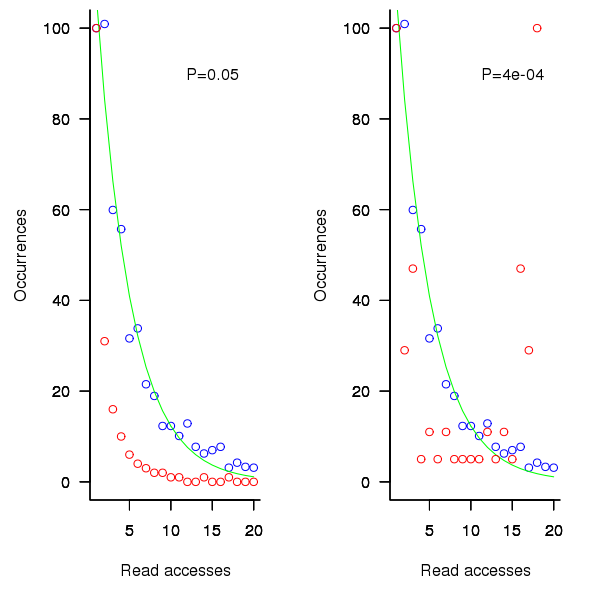
Figure 1. Variables having a given number of read accesses, given 100 total accesses, calculated from running the preferential attachment algorithm with probability of accessing a new variable at 0.05 (left, in red) and 0.0004 (right, in red), the smoothed data (blue) and a fitted exponential (green).
The results show that decreasing the probability of accessing a new variable, , does not shift the distribution of occurrences in the desired way. Note: the well known analytic solution to the outcome of running the preferential attachment algorithm, i.e., a power law, applies in the situation where the number of accesses per function definition goes to infinity.
The Preferential attachment algorithm uses a fixed probability for deciding whether to access a new variable; other measurements <book Jones_05a> imply that in practice this probability decreases as the number of distinct local variables increases. An obvious modification is to use a probability having a form something like
the number of distinct variables accessed so far). A little experimentation finds that produces results that more closely mimic the data.
While improves the fit for infrequently accessed variables, the weighting system used to select a previously accessed variable still needs attention; perhaps it also has a dependency on . Some experimentation finds that changing the probability of selection from to  (where is the number of read accesses to variable
  so far) produces behavior that matches the data to the same degree as the exponential model.
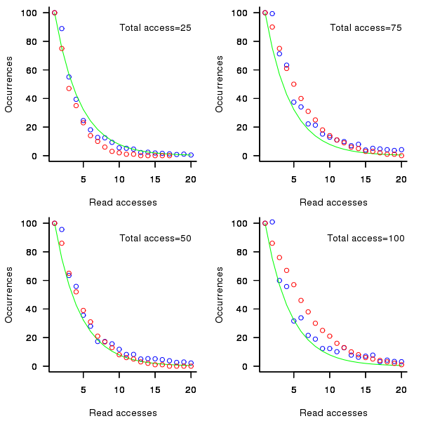
Figure 2. Variables having a given number of read accesses, given 25, 50, 75 and 100 total accesses, calculated from running the weighted preferential attachment algorithm (red), the smoothed data (blue) and a fitted exponential (green).
The weighted preferential attachment algorithm is as follows:
- With probability select a new variable to access,
- with probability
 select a variable that has previously been accessed in the function, select an existing variable with probability proportional to (where is the number of times the variable has previously been read from; e.g., if the total accesses up to this point in the code is 12, a variable that has had four previous read accesses is
  times as likely to be chosen as one that has had two previous accesses).
So what?
Both of the models are wrong in that they do not account for the small number of very frequently accessed variables that regularly occur in the data. However, as the adage goes: All models are wrong but some are useful; usefulness being evaluated by the extent to which a model solves the problem at hand. Both models have their own advantages and disadvantages, including:
- the fitted equation is quick and simple to calculate, while the output from the algorithmic model has to be averaged over many runs (1,000 are used in the example code) and is much slower,
- the algorithm automatically generates a possible sequence of accesses, while the equation does not provide an obvious way for generating a sequence of accesses,
- multiple executions of the algorithm can be used to obtain an estimate of standard deviation, while the equation does not provide a method for estimating this quantity (it may be possible to build another regression model that provides this information),
If insight into variable usage is the aim, each model provides its own particular kind of insight:
- the equation provides an end result way of thinking about how the number of variables having a given number of accesses changes, but does not provide any insight into the decision process at the level of individual accesses,
- the algorithm provides a way of thinking about how choices are made for each access, but does not provide any insight into the behavior of the final counts.
Other application domains and languages
The data used to build these models was extracted from the C source code of what might be termed desktop applications. Will the same variable access behavior characteristics occur in source written for other application domain or in other languages?
Variables might be broadly grouped into those used to hold application values (e.g., length of something) and those used to hold housekeeping values (e.g., loop counters).
Application variables are likely to be language invariant but have some dependence on algorithm (e.g., stored in an array or linked list) or cultural coding habits (e.g., within the embedded community accessing local variables is often considered to be much less efficient than accessing global variables and there are measurably different usage patterns <book Engblom_99a><book Jones 05a> figure 288.1).
The need for housekeeping values will depend on the construct supported by a language. For instance, in C loops often involve three accesses to the loop control variable to initialise, increment and test it for (i=0; i < 10; i++); in languages that support usage of the form for (i in v_list) only one access is required; in languages with vector operations many loops are implicit.
It is possible that application and language issues will change the absolute number of accesses but not effect their distribution. More measurements are needed.
Recent Comments