Archive
Impact of hardware characteristics on detectable fault behavior
Preface. This is the first of what I hope will be many posts analysing experimental data, that will eventually end up in my empirical software engineering with R book (this experiment was chosen because it happens to be the one I am currently working on; having just switched to using Asciidoc I have a backlog of editing to do on previously written analysis, also I have to figure out a way to fix [bracketed words]).
Don’t worry if you don’t know anything about the statistics used. I am aiming to provide information to meet the needs of two audiences (whether or not I fail on both counts remains to be seen):
- Those who want to some idea of what facts are known about a particular software engineering topic. Hopefully reading the introduction+conclusion will enable these readers to form an opinion about the current state of knowledge (taking my statistical analysis on trust).
- Those who are looking for ideas that can be used to analyse a problem they are trying to solve. Hopefully, somewhere among my many analyses will be something that looks like it could be applied to the reader’s problem and motivates them to go off and learn something about the statistics (if they are not already familiar with it; once written the book will obviously help out here).
Forward. The following analysis produces a negative result, something that happens a lot in experiments in all fields of research. It has been included to illustrate the importance of checking the statistical power of an experiment, i.e., how likely the experiment will detect an effect if one is present; it is very easy to fall into the trap of thinking that because lots of tests were done any effect that exists will be detected.
The authors ran an interesting experiment which as far as I know is the only published empirical analysis of intermittent software faults (please let me know if you are aware of other work) and made some mistakes in their statistical analysis. I have made plenty of mistakes in experiments I have run, some of which have found there way into the published write up. The key attribute of an experimentalist is to learn and move on.
A fault does not always noticeably change the behavior of a program when it is executed, apparently correct program execution can occur in the presence of serious faults.
A study by Syed, Robinson and Williams <book Syed_10> investigated how the number of noticeable failures caused by known faults in Mozilla’s Firefox browser varied with processor speed, system memory, hard disc size and system load. A total of 11 known faults causing intermittent failure were selected and nine different hardware configurations were selected. The conditions required to exhibit each fault were replicated and Firefox was executed 10 times for each of hardware configuration, counting the number of noticeable program failures; the seven faults and nine hardware configurations listed in the table below generated a total of 10*7*9 = 630 different executions (four faults either always or never resulted in an observed failure during the 10 runs).
Data
The following table contains the observed number of failures of Firefox for the given fault number when run on the specified hardware configuration.
| Mhz-Mb-Gb | 124750 | 380417 | 410075 | 396863 | 494116 | 264562 | 332330 |
|---|---|---|---|---|---|---|---|
|
667-128-2.5 |
4 |
10 |
6 |
5 |
2 |
3 |
5 |
|
667-256-10 |
4 |
8 |
8 |
6 |
4 |
3 |
8 |
|
667-1000-2.5 |
4 |
7 |
3 |
4 |
3 |
1 |
8 |
|
1000-128-10 |
3 |
10 |
3 |
6 |
0 |
1 |
1 |
|
1000-256-2.5 |
3 |
9 |
0 |
6 |
0 |
1 |
2 |
|
1000-1000-10 |
2 |
9 |
4 |
5 |
0 |
0 |
1 |
|
2000-128-2.5 |
0 |
10 |
5 |
6 |
0 |
0 |
0 |
|
2000-256-10 |
2 |
8 |
5 |
7 |
0 |
0 |
0 |
|
2000-1000-10 |
1 |
7 |
3 |
5 |
0 |
0 |
0 |
Predictions made in advance
There is no prior theory suggesting how the selected hardware characteristics might influence the outcome from this experiment. The analysis is based on searching for a pattern in the results and so the significance level needs to be adjusted to take account of the number of possible patterns that could exist (e.g., using the [Bonferroni correction]).
If we simplify the failure counts by labelling them as one of Low/Medium/High, then there are two arrangements of the failure counts (i.e., low/medium/high and high/medium/low) that would result in a strong correlation for cpu_speed, two arrangements for memory and two for disc size; a total of 6 combinations that would result in a strong correlation being found.
The [Bonferroni correction] adjusts the significance level by dividing by the number of tests, in this case 0.05/6 = 0.0083.
If the failure counts occurred in a random order what is the probability of a strong correlation between failure count and one of the hardware attributes being found? Based on the Low/Medium/High labelling scheme there are 9!/(3! 3! 3!) = 1680 combinations of these counts over 9 slots, giving a 1 in 1680/6 = 280 chance of purely random behavior producing a strong correlation.
The experiment investigated the characteristics of 11 faults. If there is a 1 in 280 chance of finding a strong correlation when analyzing one fault there is approximately a 1 in 24 chance of finding at least one strong correlation when analysing 11 different faults.
Response variable
The response variable takes the form of a proportion whose value varies between 0 and 1, the number of failures out of 10 executions.
Applicable techniques
The following techniques might be used to analyse this data:
- [Factorial design]. This is a way of organizing experiment configurations that is designed to extract the most information for the total number of program runs made. It would be inefficient not to use the results from some hardware configurations just because they are not needed in the factorial design and no results are available for some configurations required by a factorial design (or a [Plackett-Burman] design).
-
Fitting the data using a linear model. A standard linear model, created using R’s lm function, would not be appropriate because of the following two problems:
- this kind of model is likely to make predictions that fall outside the range 0 to 1, something that cannot happen for proportional data,
- this approach assumes that the variance is constant across measurements and unless the proportions involved are very close to each other this requirement will not be met ([proportional data] from a [binomial distribution] has variance p(1-p)).
However, a generalised linear model would not suffer from these problems. There are several [link functions] that could be used:
- the Poisson distribution, is widely used for modelling faults but requires that the mean and variance have the same value, a property that does not apply to proportional data.
- the Binomial distribution, can handle data having the characteristics present here.
The proportional data is specified in the call to the glm function by having the response variable contain two columns, one containing the number of failures (that is what is being predicted in this case) and the other the number of non-failures. The code looks something like the following (see complete example and data):
y=cbind(fail_count, 10-fail_count) glm(y ~ cpu_speed+memory+disk_size, data=ff_data, family=binomial) |
In this kind of GLM it is assumed that the [residual deviance] is the same as the [residual degrees of freedom]. If the residual deviance is greater than the residual degrees of freedom then [overdispersion] has occurred, which happens for fault 380417. To handle overdispersion the family needs to be changed from binomial to quasibinomial, which in the case of fault 380417 changes the p-value of the fit from 0.0348 to 0.0749.
The analysis of each fault finds that only one of them, 332330, has a significance level within the specified acceptable bounds; this has a negative correlation with CPU speed (i.e., observed failures decrease with clock speed).
With only one faults found to have any significant hardware configuration effects we have to ask about the probability of this experiment finding an effect if one was present.
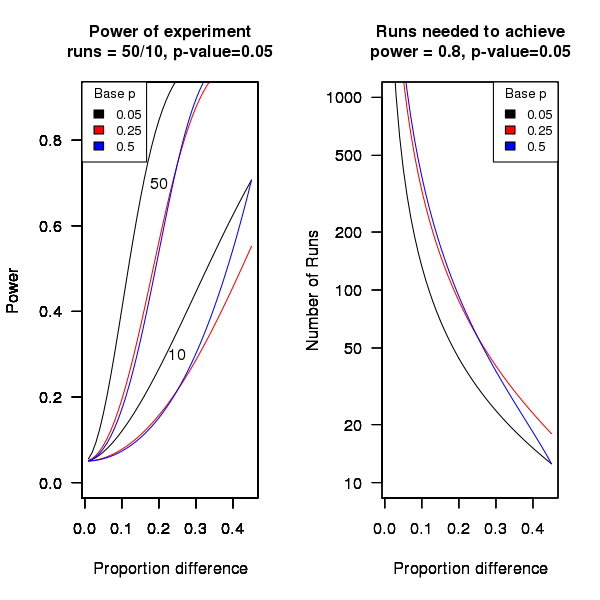
An analysis of the [statistical power] of an experiment investigating the difference between proportions for two hardware configurations (i.e., the percentage of observed failures) needs to know the value of those proportions, the number of runs (10 in this case) and the desired p-value (0.05); to simplify things the plot below is based on using the value of the lowest proportion and the difference between it and the higher proportion. The left plot shows the power achieved (y-axis) there does exist a given difference in proportions (x-axis), the three lowest proportions of 0.05, 0.25 and 0.5 are shown (the result is symmetric about 0.5 and so the plot for 0.75 and 0.95 would be the same as 0.25 and 0.05 respectively), and where there were 10 and 50 runs involving the same fault case.
It can be seen that unless a change in the hardware configuration causes a large change in the number of visible failures then the chance of a difference being detected in results from 10 runs is well below 0.5 (i.e., less than a 50% chance of detecting a difference at a p-value of 0.05 or better).
The right plot in the figure gives the number of runs that need to be made to have a 80% chance of detecting, between two different hardware configurations, the difference in proportion listed on the x-axis, at a significance of 0.05.
It can be seen that if hardware charactersitics account for only 10% of the difference in failure rate over 100 runs would be needed to detect it.
Conclusion
Faults in Firefox that caused intermittent failures were investigated looking for a correlation with system cpu speed, memory or disc size. One fault showed a strong correlation with cpu speed (there is a 1 in 24 chance that one of the investigated faults would have some kind of strong correlation). This experiment may not have found a significant correlation between observed failure rate and hardware configuration because the number of separate runs for each fault (i.e., 10) had [low power].
Trying to sell analysis tools to the Nuclear Regulatory Commission
Over the last few days there has been an interesting, and in places somewhat worrying, discussion going on in the Safety Critical mailing list about the US Nuclear Regulatory Commission. I thought I would tell my somewhat worrying story about dealing with the NRC.
In 1996 the NRC posted a request for information for a tool that I thought my company stood a reasonable chance of being able to meet (“NRC examines source code in nuclear power plant safety systems during the licensing process. NRC is interested in finding commercially available tools that can locate and provide information about the following programming practices…”). I responded, answered the questions on the form I received and was short listed to make a presentation to the NRC.
The presentation took place at the offices of National Institute of Standards and Technology, the government agency helping out with the software expertise.
From our brief email exchanges I had guessed that nobody at the NRC/NIST end knew much about C or static analysis. A typical potential customer occurrence that I was familiar with handling.
Turned up, four or so people from NRC+one(?) from NIST, gave a brief overview and showed how the tool detected the constructs they were interested in, based on test cases I had written after reading their requirements (they had not written any but did give me some code that they happened to have, that was, well, code they happened to have; a typical potential customer occurrence that I was familiar with handling).
Why did the tool produce all those messages? Well, those are the constructs you want flagged. A typical potential customer occurrence that I was familiar with handling.
Does any information have to be given to the tool, such as where to find header files (I knew that they had already seen a presentation from another tool vendor, these managers who appeared to know nothing about software development had obviously picked up this question from that presentation)? Yes, but it is very easy to configure this information… A typical potential customer occurrence that I was familiar with handling.
I asked how they planned to use the tool and what I had to do to show them that this tool met their requirements.
We want one of our inspectors to be able turn up at a reactor site and check their source code. The inspector should not need to know anything about software development and so the tool must be able to run automatically without any options being given and the output must be understandable to the inspector. Not a typical potential customer occurrence and I had no idea about how to handle it (I did notice that my mouth was open and had to make a conscious effort to keep it closed).
No, I would not get to see their final report and in fact I never heard from them again (did they find any tool vendor who did not stare at them in disbelief?)
The trip was not a complete waste of time, a few months earlier I had been at a Java study group meeting (an ISO project that ultimately failed to convince Sun to standarize Java through the ISO process) with some NIST folk who worked in the same building and I got to chat with them again.
A few hours later I realised that perhaps the question I should have asked was “What kind of software are people writing at nuclear facilities that needs an inspector to turn up and check?”
Background to my book project “Empirical Software Engineering with R”
This post provides background information that can be referenced by future posts.
For the last 18 months I have been working in fits and starts on a book that has the working title “Empirical Software Engineering with R”. The idea is to provide broad coverage of software engineering issues from an empirical perspective (i.e., the discussion is driven by the analysis of measurements obtained from experiments); R was chosen for the statistical analysis because it is becoming the de-facto language of choice in a wide range of disciplines and lots of existing books provide example analysis using R, so I am going with the crowd.
While my last book took five years to write I had a fixed target, a template to work to and a reasonably firm grasp of the subject. Empirical software engineering has only really just started, the time interval between new and interesting results appearing is quiet short and nobody really knows what statistical techniques are broadly applicable to software engineering problems (while the normal distribution is the mainstay of the social sciences a quick scan of software engineering data finds few occurrences of this distribution).
The book is being driven by the empirical software engineering rather than the statistics, that is I take a topic in software engineering and analyse the results of an experiment investigating that topic, providing pointers to where readers can find out more about the statistical techniques used (once I know which techniques crop up a lot I will write my own general introduction to them).
I’m assuming that readers have a reasonable degree of numeric literacy, are happy dealing with probabilities and have a rough idea about statistical ideas. I’m hoping to come up with a workable check-list that readers can use to figure out what statistical techniques are applicable to their problem; we will see how well this pans out after I have analysed lots of diverse data sets.
Rather than wait a few more years before I can make a complete draft available for review I have decided to switch to making available individual parts as they are written, i.e., after writing a draft discussion and analysis of each experiment I will published it on this blog (along with the raw data and R code used in the analyse). My reasons for doing this are:
- Reader feedback (I hope I get some) will help me get a better understanding of what people are after from a book covering empirical software engineering from a statistical analysis of data perspective.
- Suggestions for topics to cover. I am being very strict and only covering topics for which I have empirical data and can make that data available to readers. So if you want me to cover a topic please point me to some data. I will publish a list of important topics for which I currently don’t have any data, hopefully somebody will point me at the data that can be used.
- Posting here will help me stay focused on getting this thing done.
Links to book related posts
Distribution of uptimes for high-performance computing systems
Break even ratios for development investment decisions
Agreement between code readability ratings given by students
Changes in optimization performance of gcc over time
Descriptive statistics of some Agile feature characteristics
Impact of hardware characteristics on detectable fault behavior
Prioritizing project stakeholders using social network metrics
Preferential attachment applied to frequency of accessing a variable
Amount of end-user usage of code in Firefox
How many ways of programming the same specification?
Ways of obtaining empirical data in software engineering
What is the error rate for published mathematical proofs?
Changes in the API/non-API method call ratio with program size
Honking the horn for go faster memory (over go faster cpus)
How to avoid being a victim of Brooks’ law
Evidence for the benefits of strong typing, where is it?
Hardware variability may be greater than algorithmic improvement
Extracting the original data from a heatmap image
Entropy: Software researchers go to topic when they have no idea what else to talk about
Maths GCE from 1972 (paper 2)
While sorting through some old papers I came across my GCE maths O level exam papers from the summer of 1972. They are known as GCSE exams these days and are taken by 16 year olds at the end of their final year of compulsory education in the UK. I was lucky enough to have a maths teacher who believed in encouraging students to excel and I (plus five others) took this exam when we were 15. I never got the chance to thank Mr Merritt for the profound effect he had on my life.
For many years the average grades achieved by students in the UK has had a steady upward trend and some people claim the exams are getting easier (others that students are better taught, or at least better taught to pass exams). These days students have calculators and don’t use log tables, so question 3 of Section A is not applicable.
Exam papers in the UK are written by various examining boards. Mine were from the University of London, Syllabus D. I have two papers labeled “Mathematics 2” and “Mathematics 3” and don’t recall if there was ever a “Mathematics 1”. The following are the questions from “Mathematics 2”.
All necessary working must be shown.
- Factorise

Hence, or otherwise, find the exact value of
")
4 marks
- Given that
}") , express
, express  in terms of
  and
and  .
.
3 marks
- Use four digit tables to evaluate
}") .
.
4 marks
- Given that
 is a factor of
  , calculate the value of
  .
.
3 marks
-

In the diagram ∠DBC = ∠BAD and ADC is a straight line. State which of the two triangles are similar.
If AB = 7 cm, BC = 6 cm and DC = 4 cm, calculate the lengths of AC and BD.
5 marks
- A bicycle wheel has diameter 35 cm. Calculate how many revolutions it makes every minute when the bicycle is travelling at 33 km/h. [ Take
 as 22/7 ]
4 marks
- Calculate the gradient of the curve
 at the point (1, -5). Calculate also the coordinates of the point on the curve where the gradient is 1.
4 marks
-
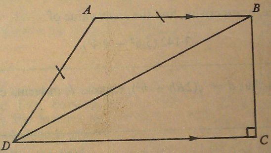
In the diagram, AB is parallel to DC, AB = AD and ∠C = 90°. Prove that ∠DAB = 2∠DBC.
5 marks
as 3.142 when required- A ship is at the point P (54°N, 55°W). Calculate the distance, in nautical miles, of P from the equator.
The ship then sails 500 nautical miles due East to a point Q. Calculate the latitude and longitude of Q.
An aircraft flies due South at a constant height of 10 000 m from the point vertically above P to a point vertically above the equator. Taking the earth to be a sphere of radius 6 370 km, calculate the length of the arc along which the aircraft flies.
17 marks
- Draw a circle of radius 5.5 cm. Using ruler and compasses only, construct a tangent to the circle at any point A on its circumference.
Using a protractor, construct the points A, B and C on this circle so that the angles A, B and C of the triangle ABC are 50°, 56° and 74° respectively.
By a further construction using ruler and compasses only, obtain a point X on the tangent at A which is equidistant from the lines AB and BC.
Measure the length of AX.
17 marks
- (i) Find the smallest positive term in the arithmetic progression 76, 74½, 73 … .
Find also the number of positive terns in the progression and the sum of these positive terms.
(ii) The first and fourth terms in a geometric progression are
 and
and  respectively. Find the second and third terms of the progression.
17 marks
-
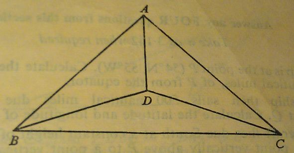
The diagram represents a roof-truss in which AB = AC = 8 m, BC = 11 m, BD = DC and ∠DBC = 20°.
Calculate
(a) the length BD,
(b) the angle ABC,
(c) the length AD.
- Draw the graph of
 for values of
  from -1 to +4, taking 2 cm as one unit on the x-axis and 1 cm as one unit on the y-axis. From your graph, find the range of values of for which the function
  is greater than 6.
Using the sane axes and scales, draw the graph of
 and write down the coordinates of the points of intersection of the two graphs.
if
 is the quadratic equation of which these coordinates are the roots, determine the values of
  and
and  .
.17 marks
- A particle starts from rest at a point A and moves along a straight line, coming to rest again at another point B. During the motion its velocity,
 metres per second, after time
  is given by
  .
.
Calculate:
(a) the time taken for the particle to reach B.
(b) the distance travelled during the first two seconds,
(c) the time taken for the particle to attain its maximum velocity,
(d) the maximum velocity attained,
(e) the maximum acceleration during the motion.
17 marks
Automatically generating railroad diagrams from yacc files
Reading and understanding a language’s syntax written in the BNF-like notation used by yacc/bison takes some practice. Railroad diagrams are a much more user friendly notation, but require a lot of manual tweaking before they look as good as the following example from the json.org website:
I’m currently working on a language whose syntax is evolving and I want to create a visual representation of it that can be read by non-yacc experts; spending a day of so manually creating a decent looking railroad diagram is not an efficient use of time. What automatic visualization tools are out there that I can use?
A couple of tools that look like they might produce useful results are web based (e.g., bottlecaps.de; working on an internal project for a company means I cannot take this approach). Some tools take EBNF as input (e.g., my28msec.com which is also online based); the Extensions in EBNF obviate the need for many of the low level organizational details that appear in grammars written with BNF, making grammars written using EBNF easier to layout and look good; great if I was working with EBNF. The yacc file input tools I tried (yaccviso, Vyacc) were a bit too fragile and the output was not that good.
Bison has an option to generate a output that can be processed into graphical form (using graphviz as the layout engine). Unfortunately the graphs produced are as visually tangled as the input grammar and if anything harder to follow.
It is possible to produce great looking visual diagrams using a simple tool if you are willing to spend lots of fiddling with the input grammar to control the output. I wanted to take the grammar as written (i.e., a yacc input file) and am willing to accept less than perfect output.
Most of the syntax rules in a yacc grammar are straight forward sequences of tokens that have an obvious one-to-one mapping and there are a few commonly seen idioms. I decided to write a tool that concentrated on untangling the idioms and let the simple stuff look after itself. One idiom that has a visual representation very different from its yacc form is the two productions used to specify an arbitrary long list, e.g., a semicolon separated list of ys is often written as (ok, there might perhaps be times when right recursion is appropriate):
x : y | x ";" y ; |
and I wanted something that looked like (from the sql-lite web site, which goes one better and allows support for the list to be optional:
Graph layout is a complicated business and like everybody else I decided to use graphviz to do the heavy lifting (specifically I would generate the layout directives used by dot). All I had to do was write a yacc grammar to dot translator (and not spend lots of time doing it).
The dot language provides a directives that specify the visual properties of nodes and the connections between them. For instance:
n_0[shape=point] n_1[label="sql-stmt"] n_2[label=";"] n_3[shape=point] n_0 -> n_3 n_0 -> n_1 n_1 -> n_3 n_1 -> n_2 n_2 -> n_1 |
is the dot specification of the optional semicolon separated list of sql-stmts displayed above.
Dot takes a list of directives describing the nodes and edges of a graph and makes its own decisions about how to layout the output. It is possible to specify in excruciating detail exactly how to do the layout, but I wanted everything to be automated.
I decided to write the tool in awk because it has great input token handling facilities and I use it often enough to be fluent.
Each grammar rule containing one or more productions is mapped to a single graph. When generating postscript dot puts each graph on a separate page, other output formats appear to loose all but one of the graphs. To make sure each rule fitted on a page I had the text point size depend on the number of productions in a rule, more productions smaller point size. The most common idioms are handled (i.e., list-of and optional construct) with hooks available to handle others. Productions within a rule will often have common token sequences but the current version only checks for matching token sequences at the start of a production and all productions in a rule have to start with the same sequence. Words written all in upper-case are assumed to be language tokens and are converted to lower case and bracketed with quotes. The 300+ lines of conversion tool’s awk source is available for download.
The follow examples are taken from an attempted yacc grammar of C++ done when people still thought such a thing could be created. While the output does have a certain railroad diagram feel to it, the terrain must be very hilly to generate those curvaceous lines.
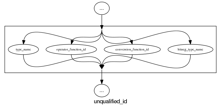
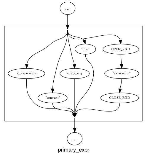
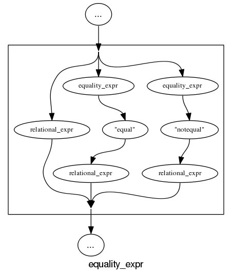
and the run of the mill rules look good, a C++ primary-expression is:
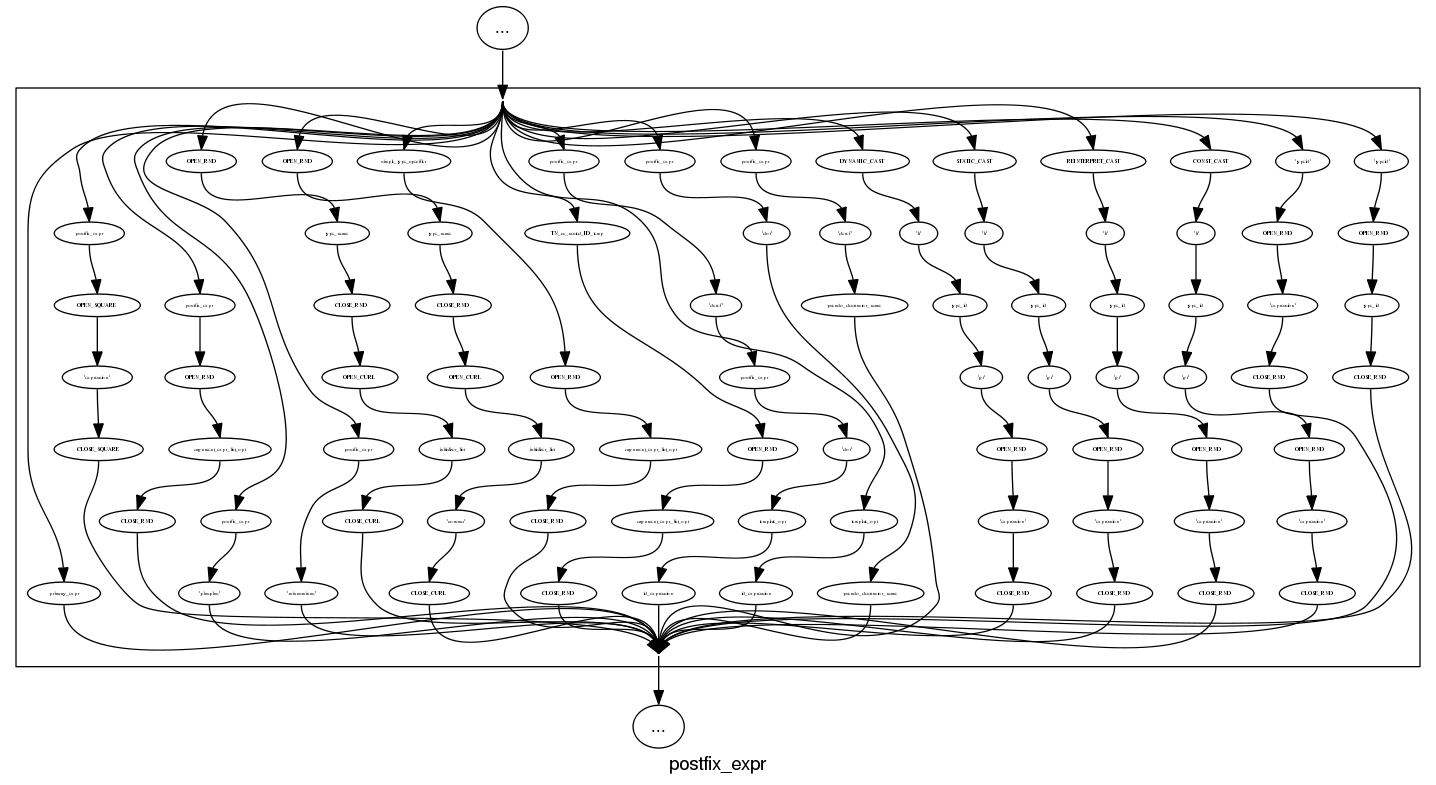
and we can rely on C++ to push syntax rule complexity to the limit, a postfix-expression is:
What about the idioms? A simple list of items looks good:
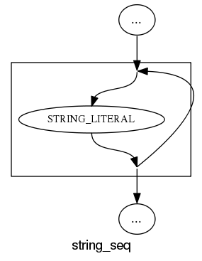
and slightly less good when separators are involved:
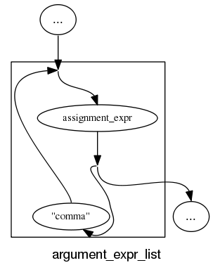
and if we push our luck things start to look tangled:
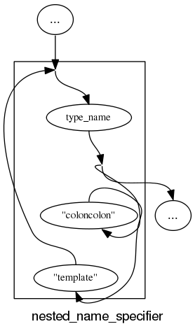
With a bit more work invested on merging token sequences common to two or more rules the following might look a lot less cluttered:
Apart from a few tangled cases the results are not bad for a tool that was a few hours work. I will wait a bit to see if the people I deal with find this visual form of use.
In the meantime I would be interested to hear about my readers experience with visualizing grammars, using dot to this kind of thing and any suggestions they have. As a long time user of dot I know that there are lots of ways of influencing the final layout (e.g., changing the ordering or edges and nodes in its input), I will have to be careful not to get pulled down this rabbit hole.
Why do companies fix faults in software they sell?
Once I buy some software from a company they have my money, if sometime later I find a fault software what incentive does that company have to fix the software and provide me with an update (assuming the software is not so fault ridden that I take advantage of laws allowing me to return a purchase for a refund)?
There are three economic incentives for companies to fix faults:
- because I am paying them a fee for updates that include fixes to known faults,
- because they want to make future sales to me and to others (faults encountered by customers contribute towards the perception of product quality),
- they don’t want to lose money because a fault had consequences that resulted in legal action (this reason is overhyped, in practice software engineering has a missing dead body problem).
Which faults get fixed? Software is surprisingly fault-tolerant and there is no point in fixing faults that customers are unlikely to encounter. This means that once a product has been released and known to be acceptable to many customers, there is no incentive to actively search for faults; this means that the only faults likely to be fixed are the ones reported by customers.
When reporting a fault, customers are often asked to rate its severity. This is a useful technique for prioritizing what gets fixed first, or perhaps what does not get fixed at all. Customers who actively set out to find faults are not appreciated and are labelled as disruptive if they continue doing it. Finding faults is surprisingly easy, finding the faults that have a high probability of being encountered by customers and ranked by them as critical is very hard (this is one of the reasons static analysis tools are not widely used).
What is the motivation for developers to fix faults in Open Source?
- There are companies who provide support services for a fee, just like commercial offerings,
- Open Source is free, gaining more users is not an obvious incentive to fix faults. However, being known as the go-to guys for a given package is a way of attracting companies looking to hire somebody to provide support services or make custom modifications to that package. Fixing faults is a way of getting visibility, it is advertising.
- Developers hate the thought of doing something wrong resulting in a fault in code they have written, and writing faulty code is not socially acceptable behavior in software development circles. These feelings about what constitutes appropriate behavior are often enough to make developers want to spend time fixing faults in code they have written or feel responsible for, provided they have the time. I suspect a lot of faults get fixed by developers when their manager/wife thinks they are working on something more ‘useful’.
Recent Comments