Archive
Fitting discontinuous data from disparate sources
Sorting and searching are probably the most widely performed operations in computing; they are extensively covered in volume 3 of The Art of Computer Programming. Algorithm performance is influence by the characteristics of the processor on which it runs, and the size of the processor cache(s) has a significant impact on performance.
A study by Khuong and Morin investigated the performance of various search algorithms on 46 different processors. Khuong The two authors kindly sent me a copy of the raw data; the study webpage includes lots of plots.
The performance comparison involved 46 processors (mostly Intel x86 compatible cpus, plus a few ARM cpus) times 3 array datatypes times 81 array sizes times 28 search algorithms. First a 32/64/128-bit array of unsigned integers containing N elements was initialized with known values. The benchmark iterated 2-million times around randomly selecting one of the known values, and then searching for it using the algorithm under test. The time taken to iterate 2-million times was recorded. This was repeated for the 81 values of N, up to 63,095,734, on each of the 46 processors.
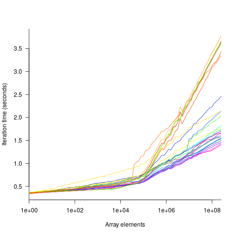
The plot below shows the results of running each algorithm benchmarked (colored lines) on an Intel Atom D2700 @ 2.13GHz, for 32-bit array elements; the kink in the lines occur roughly at the point where the size of the array exceeds the cache size (all code+data):
What is the most effective way of analyzing the measurements to produce consistent results?
One approach is to build two regression models, one for the measurements before the cache ‘kink’ and one for the measurements after this kink. By adding in a dummy variable at the kink-point, it is possible to merge these two models into one model. The problem with this approach is that the kink-point has to be chosen in advance. The plot shows that the performance kink occurs before the array size exceeds the cache size; other variables are using up some of the cache storage.
This approach requires fitting 46*3=138 models (I think the algorithm used can be integrated into the model).
If data from lots of processors is to be fitted, or the three datatypes handled, an automatic way of picking where the first regression model should end, and where the second regression model should start is needed.
Regression discontinuity design looks like it might be applicable; treating the point where the array size exceeds the cache size as the discontinuity. Traditionally discontinuity designs assume a sharp discontinuity, which is not the case for these benchmarks (R’s rdd package worked for one algorithm, one datatype running on one processor); the more recent continuity-based approach supports a transition interval before/after the discontinuity. The R package rdrobust supports a continued-based approach, but seems to expect the discontinuity to be a change of intercept, rather than a change of slope (or rather, I could not figure out how to get it to model a just change of slope; suggestions welcome).
Another approach is to use segmented regression, i.e., one of more distinct lines. The package segmented supports fitting this kind of model, and does estimate what they call the breakpoint (the user has to provide a first estimate).
I managed to fit a segmented model that included all the algorithms for 32-bit data, running on one processor (code+data). Looking at the fitted model I am not hopeful that adding data from more than one processor would produce something that contained useful information. I suspect that there are enough irregular behaviors in the benchmark runs to throw off fitting quality.
I’m always asking for more data, and now I have more data than I know how to analyze in a way that does not require me to build 100+ models 🙁
Suggestions welcome.
Building a regression model is easy and informative
Running an experiment is very time-consuming. I am always surprised that people put so much effort into gathering the data and then spend so little effort analyzing it.
The Computer Language Benchmarks Game looks like a fun benchmark; it compares the performance of 27 languages using various toy benchmarks (they could not be said to be representative of real programs). And, yes, lots of boxplots and tables of numbers; great eye-candy, but what do they all mean?
The authors, like good experimentalists, make all their data available. So, what analysis should they have done?
A regression model is the obvious choice and the following three lines of R (four lines if you could the blank line) build one, providing lots of interesting performance information:
cl=read.csv("Computer-Language_u64q.csv.bz2", as.is=TRUE)

cl_mod=glm(log(cpu.s.) ~ name+lang, data=cl)
summary(cl_mod) |
The following is a cut down version of the output from the call to summary, which summarizes the model built by the call to glm.
                    Estimate Std. Error t value Pr(>|t|)
(Intercept)         1.299246   0.176825   7.348 2.28e-13 ***
namechameneosredux  0.499162   0.149960   3.329 0.000878 ***
namefannkuchredux   1.407449   0.111391  12.635  < 2e-16 ***
namefasta           0.002456   0.106468   0.023 0.981595
namemeteor         -2.083929   0.150525 -13.844  < 2e-16 ***

langclojure         1.209892   0.208456   5.804 6.79e-09 ***
langcsharpcore      0.524843   0.185627   2.827 0.004708 **
langdart            1.039288   0.248837   4.177 3.00e-05 ***
langgcc            -0.297268   0.187818  -1.583 0.113531
langocaml          -0.892398   0.232203  -3.843 0.000123 ***

    Null deviance: 29610  on 6283  degrees of freedom
Residual deviance: 22120  on 6238  degrees of freedom
What do all these numbers mean?
We start with glm's first argument, which is a specification of the regression model we are trying to fit: log(cpu.s.) ~ name+lang
cpu.s. is cpu time, name is the name of the program and lang is the language. I found these by looking at the column names in the data file. There are other columns in the data, but I am running in quick & simple mode. As a first stab, I though cpu time would depend on the program and language. Why take the log of the cpu time? Well, the model fitted using cpu time was very poor; the values range over several orders of magnitude and logarithms are a way of compressing this range (and the fitted model was much better).
The model fitted is:
 , or
, or 
Plugging in some numbers, to predict the cpu time used by say the program chameneosredux written in the language clojure, we get:  (values taken from the first column of numbers above).
This model assumes there is no interaction between program and language. In practice some languages might perform better/worse on some programs. Changing the first argument of glm to: log(cpu.s.) ~ name*lang, adds an interaction term, which does produce a better fitting model (but it's too complicated for a short blog post; another option is to build a mixed-model by using lmer from the lme4 package).
We can compare the relative cpu time used by different languages. The multiplication factor for clojure is  , while for
 ocaml it is  . So
. So clojure consumes 8.2 times as much cpu time as ocaml.
How accurate are these values, from the fitted regression model?
The second column of numbers in the summary output lists the estimated standard deviation of the values in the first column. So the clojure value is actually }") , i.e., between 2.2 and 4.9 (the multiplication by 1.96 is used to give a 95% confidence interval); the
, i.e., between 2.2 and 4.9 (the multiplication by 1.96 is used to give a 95% confidence interval); the ocaml values are }") , between 0.3 and 0.6.
, between 0.3 and 0.6.
The fourth column of numbers is the p-value for the fitted parameter. A value of lower than 0.05 is a common criteria, so there are question marks over the fit for the program fasta and language gcc. In fact many of the compiled languages have high p-values, perhaps they ran so fast that a large percentage of start-up/close-down time got included in their numbers. Something for the people running the benchmark to investigate.
Isn't it easy to get interesting numbers by building a regression model? It took me 10 minutes, ok I spend a lot of time fitting models. After spending many hours/days gathering data, spending a little more time learning to build simple regression models is well worth the effort.
Uncertainty in data causes inconsistent models to be fitted
Does software development benefit from economies of scale, or are there diseconomies of scale?
This question is often expressed using the equation:  . If
. If  is less than one there are economies of scale, greater than one there are diseconomies of scale. Why choose this formula? Plotting project effort against project size, using logs scales, produces a series of points that can be sort-of reasonably fitted by a straight line; such a line has the form specified by this equation.
Over the last 40 years, fitting a collection of points to the above equation has become something of a rite of passage for new researchers in software cost estimation; values for have ranged from 0.6 to 1.5 (not a good sign that things are going to stabilize on an agreed value).
This article is about the analysis of this kind of data, in particular a characteristic of the fitted regression models that has been baffling many researchers; why is it that the model fitted using the equation is not consistent with the model fitted using  , using the same data. Basic algebra requires that the equality
  be true, but in practice there can be large differences.
The data used is Data set B from the paper Software Effort Estimation by Analogy and Regression Toward the Mean (I cannot find a pdf online at the moment; Code+data). Another dataset is COCOMO 81, which I analysed earlier this year (it had this and other problems).
The difference between and  is a result of what most regression modeling algorithms are trying to do; they are trying to minimise an error metric that involves just one variable, the response variable.
In the plot below left a straight line regression has been fitted to some Effort/Size data, with all of the error assumed to exist in the  values (dotted red lines show the residual for each data point). The plot on the right is another straight line fit, but this time the error is assumed to be in the
  values (dotted green lines show the residual for each data point, with red line from the left plot drawn for reference). Effort is measured in hours and Size in function points, both scales show the
  of the actual value.
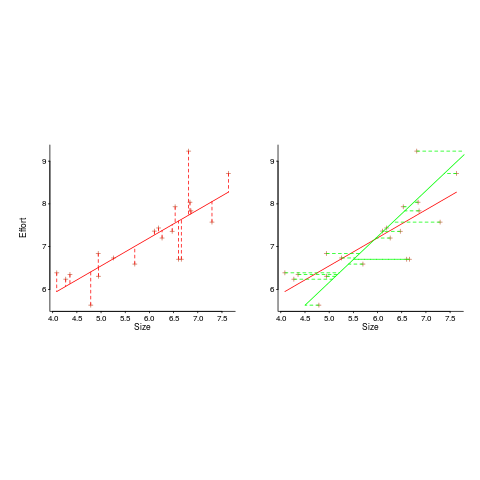
Regression works by assuming that there is NO uncertainty/error in the explanatory variable(s), it is ALL assumed to exist in the response variable. Depending on which variable fills which role, slightly different lines are fitted (or in this case noticeably different lines).
Does this technical stuff really make a difference? If the measurement points are close to the fitted line (like this case), the difference is small enough to ignore. But when measurements are more scattered, the difference may be too large to ignore. In the above case, one fitted model says there are economies of scale (i.e.,  ) and the other model says the opposite (i.e.,
  , diseconomies of scale).
There are several ways of resolving this inconsistency:
- conclude that the data contains too much noise to sensibly fit a a straight line model (I think that after removing a couple of influential observations, a quadratic equation might do a reasonable job; I know this goes against 40 years of existing practice of do what everybody else does…),
- obtain information about other important project characteristics and fit a more sophisticated model (characteristics of one kind or another are causing the variation seen in the measurements). At the moment information is being used to explain all of the variance in the data, which cannot be done in a consistent way,
- fit a model that supports uncertainty/error in all variables. For these measurements there is uncertainty/error in both and ; writing the same software using the same group of people is likely to have produced slightly different Effort/Size values.
There are regression modeling techniques that assume there is uncertainty/error in all variables. These are straight forward to use when all variables are measured using the same units (e.g., miles, kilogram, etc), but otherwise require the user to figure out and specify to the model building process how much uncertainty/error to attribute to each variable.
In my Empirical Software Engineering book I recommend using simex. This package has the advantage that regression models can be built using existing techniques and then ‘retrofitted’ with a given amount of standard deviation in specific explanatory variables. In the code+data for this problem I assumed 10% measurement uncertainty, a number picked out of thin air to sound plausible (its impact is to fit a line midway between the two extremes seen in the right plot above).
Converting between IFPUG & COSMIC function point counts
Replication, repeating an experiment to confirm the results of previous experiments, is not a common activity in software engineering. Everybody wants to write about their own ideas and academic journals want to publish what is new (they are fashion driven).
Conversion between ways of counting function points, a software effort estimating technique, is one area where there has been a lot of replications (eight studies is a lot in software engineering, while a couple of hundred is a lot in psychology).
Amiri and Padmanabhuni’s Master’s thesis (yes, a thesis written by two people) lists data from 11 experiments where students/academics/professionals counted function points for a variety of projects using both the IFPUG and COSMIC counting methods. The data points are plotted below left and regression lines to each sample on the right (code+data):
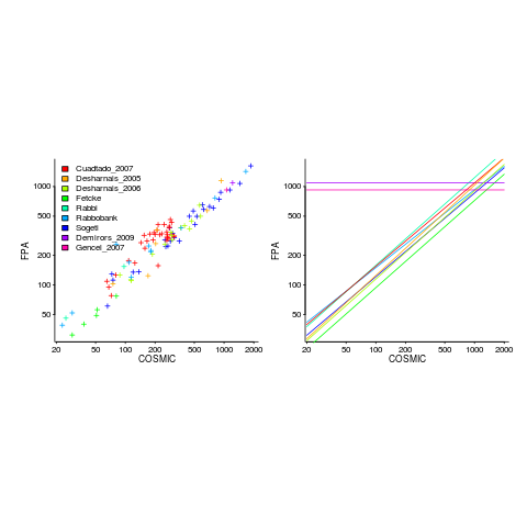
The horizontal lines are two very small samples where model fitting failed.
I was surprised to see such good agreement between different groups of counters. A study by Grimstad and Jørgensen asked developers to estimate effort (not using function points) for various projects, waited one month and repeated using what the developers thought were different projects. Most of the projects were different from the first batch, but a few were the same. The results showed developers giving completely different estimates for the same project! It looks like the effort invested in producing function point counting rules that give consistent answers and the training given to counters has paid off.
Two patterns are present in the regression lines:
- the slope of most lines is very similar, but they are offset from each other,
- the slope of some lines is obviously different from the others, with the different slopes all tilting further in the same direction. These cases mostly occur in the Cuadrado data (these three data sets are not included in the following analysis).
The kind of people doing the counting, for each set of measurements, is known and this information can be used to build a more sophisticated model.
Specifying a regression model to fit requires making several decisions about the kinds of uncertainty error present in the data. I have no experience with function points and in the following analysis I list the options and pick the one that looks reasonable to me. Please let me know if you have theory or data one suggesting what the right answer might be, I’m just juggling numbers here.
First we have to decide whether measurement error is additive or multiplicative. In other words, is there a fixed amount of potential error on each measurement, or is the amount of error proportional to the size of the project being measured (i.e., the error is a percentage of the total).
Does it make a difference to the fitted model? Sometimes it does and its always worthwhile to try building a model that mimics reality. If I tell you that  (Greek lower-case epsilon) is the symbol used to denote measurement error, you should be able to figure out which of the following two equations was built assuming additive/multiplicative error (confidence intervals have been omitted to keep things simple, they are given at the end of this post).
log(CFP)}*e^{0.81IFPi-0.6CFPi}*e^{0.24stu}+epsilon")
log(CFP)}*e^{0.83IFPi}*e^{0.29stu}*epsilon")
where:  is 0 when the IFPUG counting is done by academics and 1 when done by industry,
  is 0 when the COSMIC counting is done by academics and 1 when done by industry,
  is 1 when the counting was done by students and 0 otherwise.
I think that measurement error is multiplicative for his problem and the remaining discussion is based on this assumption. Everything after the first exponential can be treated as effectively a constant, say  , giving:
log(CFP)}*K")
If we are only interested in converting counts performed by industry we get:

If we are using academic counters the equation is:

Next we have to decide where the uncertainty error resides. Nearly all forms of regression modeling assume that all the uncertainty resides in the response variable and that there is no uncertainty in the explanatory variables are measured without uncertainty. The idea is that the values of the explanatory variables are selected by the person doing the measurement, a handle gets turned and out pops the value of the response variable, plus error, for those particular, known, explanatory variable.
The measurements in this analysis were obtained by giving the subjects a known project specification, getting them to turn a handle and recording the function point count that popped out. So all function point counts contain uncertainty error.
Does the choice of response variable make that big a difference?
Let’s take the model fitted above and do some algebra to invert it, so that COSMIC is expressed in terms of IFPUG. We get the equation:

Now lets fit a model where the roles of response/explanatory variable are switched, we get:

For this problem we need to fit a model that includes uncertainty in both variables containing function point counts. There are techniques for building models from scratch, known as errors-in-variables models. I like the SIMEX approach because it integrates well with existing R functionality for building regression models.
To use the simex function, from the R simex package, I have to decide how much uncertainty (in the form of a value for standard deviation) is present in the explanatory variable (the COSMIC counts in this case). Without any knowledge to guide the choice, I decided that the amount of error in both sets of count measurements is the same (a standard deviation of 3%, please let me know if you have a better idea).
The fitted equation for a model containing uncertainty in both counts is (see code+data for model details):

If I am interested in converting IFPUG counts to COSMIC, then what is the connection between the above model and reality?
I’m guessing that those most likely to perform conversions are in industry. Does this mean we can delete the academic subexpressions from the model, or perhaps fit a model that excludes counts made by academics? Is the Cuadrado data sufficiently different to be treated as an outlier than should be excluded from the model building process, or is it representative of an industry usage that does not occur in the available data?
There are not many industry only counts in the combined data. Perhaps the academic counters are representative of counters in industry that happen not to be included in the samples. We could build a mixed-effects model, using all the data, to get some idea of the variation between different sets of counters.
The 95% confidence intervals for the fitted exponent coefficient, using this data, is around 8%. So in practice, some of the subtitles in the above analysis are lost in the noise. To get tighter confidence bounds more data is needed.
Ordinary Least Squares is dead to me
Most books that discuss regression modeling start out and often finish with Ordinary Least Squares (OLS) as the technique to use; Generalized Linear ModelLeast Squares (GLMS) sometimes get a mention near the back. This is all well and good if the readers’ data has the characteristics required for OLS to be an applicable technique. A lot of data in the social sciences has these characteristics, or so I’m told; lots of statistics books are written for social science students, as a visit to a bookshop will confirm.
Software engineering datasets often range over several orders of magnitude or involve low value count data, not the kind of data that is ideally suited for analysis using OLS. For this kind of data GLMS is probably the correct technique to use (the difference in the curves fitted by both techniques is often small enough to be ignored for many practical problems, but the confidence bounds and p-values often differ in important ways).
The target audience for my book, Empirical Software Engineering with R, are working software developers who have better things to do that learn lots of statistics. However, there is no getting away from the fact that I am going to have to make extensive use of GLMS, which means having to teach readers about the differences between OLS and GLMS and under what circumstances OLS is applicable. What a pain.
Then I had a brainwave, or a moment of madness (time will tell). Why bother covering OLS? Why not tell readers to always use GLMS, or rather use the R function that implements it, glm. The default glm behavior is equivalent to lm (the R function that implements OLS); the calculation is not being done by hand but by a computer (i.e., who cares if it is more complicated).
Perhaps there is an easy way to explain this to software developers: glm is the generic template that can handle everything and lm is a specialized template that is tuned to handle certain kinds of data (the exact technical term will need tweaking for different languages).
There is one user interface issue, models built using glm do not come with an easy to understand goodness of fit number (lm has the R-squared value). AIC is good for comparing models but as a single (unbounded) number it is not that helpful for the uninitiated. Will the demand for R-squared be such that I will be forced for tell readers about lm? We will see.
How do I explain the fact that so many statistics books concentrate on OLS and often don’t mention GLMS? Hey, they are for social scientists, software engineering data requires more sophisticated techniques. I will have to be careful with this answer as it plays on software engineers’ somewhat jaded views of social scientists (some of whom have made very major contribution to CRAN).
All the software engineering data I have seen is small enough that the performance difference between glm/lm is not a problem. If performance is a real issue then readers will search the net and find out about lm; sorry guys but I want to minimise what the majority of readers need to know.
Recent Comments