Archive
Distribution of small project completion times
Records of project estimates and actual task times show that round numbers are very common. Various possible reasons have been suggested for why actual times are often reported as a round number. This post analyses the impact of round number reports of actual times on the accuracy of estimates.
The plot below shows the number of tasks having a given reported completion time for 1,525 tasks estimated to take 1-hour (code+data):
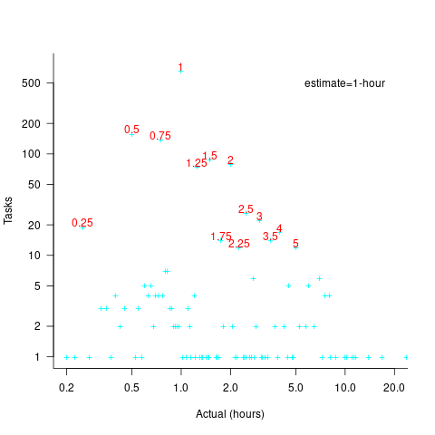
Of those 1,525 tasks estimated to take 1-hour, 44% had a reported completion time of 1-hour, 26% took less than 1-hour and 30% took more than 1-hour. The mean is 1.6 hours and the standard deviation 7.1. The spikiness of the distribution of actual times rules out analytical statistical analysis of the distribution.
If a large task is broken down into, say,  smaller tasks, all estimated to take the same amount of time
  , what is the distribution of actual times for the large task?
In the case of just two possible actual times to complete each smaller task, some percentage,  , of tasks are completed in actual time
  , and some percentage,
  , completed in actual time
  (with
(with  ). The probability distribution of the large task time,
 ") , for the two actual times case is:
, for the two actual times case is:
=(matrix{2}{1}{N k})(1-p_{t1})^k {p_{t1}}^{N-k}=(matrix{2}{1}{N k}){p_{t2}}^k (1-p_{t2})^{N-k}")
where:  , and
, and  .
.
The right-most equation is the probability distribution of the Binomial distribution, ") . The possible completion times for the large task start at
. The possible completion times for the large task start at  , followed by time increments of .
When there are three possible actual completion times for each smaller task, the calculation is complicated, and become more complicated with each new possible completion time.
A practical approach is to use Monte Carlo simulation. This involves simulating lots of large tasks containing smaller tasks. A sample of tasks is randomly drawn from the known 1,525 task actual times, and these actual times added to give one possible completion time. Running this process, say, 10,000 times produces what is known as the empirical distribution for the large task completion time.
The plot below shows the empirical distribution  smaller 1-hour tasks. The blue/green points show two peaks, the higher peak is a consequence of the use of round numbers, and the lower peak a consequence of the many non-round numbers. If the total times are rounded to 15 minute times, red points, a smoother distribution with a single peak emerges (code+data):

When a large task involves smaller tasks estimated to take a variety of times, the empirical distribution of the actual time for each estimated time can be combined to give an empirical distribution of the large task (see sum_prob_distrib).
Provided enough information on task completion times is available, this technique works does what it says on the tin.
Distribution of binary operator results
As numeric values percolate through a program they appear as the operands of arithmetic operators whose results are new values. What is the distribution of binary operator result values, for a given distribution of operand values?
If we start with independent random values drawn from a uniform distribution,  , then:
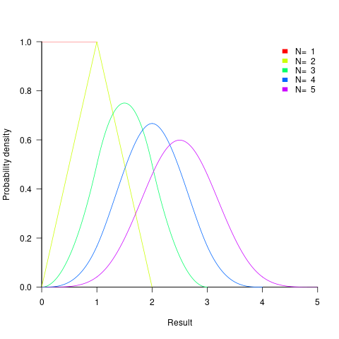
- the distribution of the result of adding two such values has a triangle distribution, and the result distribution from adding such values is known as the Irwin-Hall distribution (a polynomial whose highest power is
 ). The following plot shows the probability density of the result of adding 1, 2, 3, 4, and 5 such values (code+data):
- the distribution of the result of multiplying two such values has a logarithmic distribution, and when multiplying such values the probability of the result being
 is:
is: ^{N-1}/{(N-1)!}") .
.
If the operand values have a lognormal distribution, then the result also has a lognormal distribution. It is sometimes possible to find a closed form expression for operand values having other distributions.
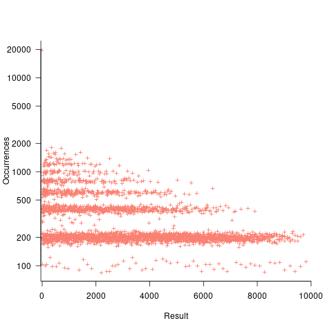
If both operands take integer values, including zero, some result values are more likely to occur than others; for instance, there are six unique factor pairs of positive integers that when multiplied return sixty, and of course prime numbers only have one factor-pair. The following plot was created by randomly generating one million pairs of values between 0 and 100 from a uniform distribution, multiplying each pair, and counting the occurrences of each result value (code+data):
- the probability of the result of dividing two such values being is: 0.5 when
 , and
, and  when
when  .
.
The ratio of two distributions is known as a ratio distribution. Given the prevalence of Normal distributions, their ratio distribution is of particular interest, it is a Cauchy distribution:
}") ,
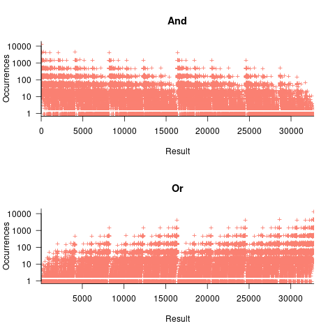
, - the result distribution of the bitwise and/or operators is not continuous. The following plots were created by randomly generating one million pairs of values between 0 and 32,767 from a uniform distribution, performing a bitwise AND or OR, and counting the occurrences of each value (code+data):
- the result distribution of the bitwise exclusive-or operator is uniform, when the distribution of its two operands is uniform.
The mean value of the Irwin-Hall distribution is  and its standard deviation is
  . As
. As  , the Irwin-Hall distribution converges to the Normal distribution; the difference between the distributions is approximately:
 ^N") .
.
The sum of two or more independent random variables is the convolution of their individual distributions,
The banding around intervals of 100 is the result of values having multiple factor pairs. The approximately 20,000 zero results are from two sets of  multiplications where one operand is zero,
The vertical comb structure is driven by power-of-two bits being set/or not. For bitwise-and the analysis is based on the probability of corresponding bits in both operands being set, e.g., there is a 50% chance of any bit being set when randomly selecting a numeric value, and for bitwise-and there is a 25% chance that both operands will have corresponding bits set; numeric values with a single-bit set are the most likely, with two bits set the next most likely, and so on. For bitwise-or the analysis is based on corresponding operand bits not being set,
The general pattern is that sequences of addition produce a centralizing value, sequences of multiplies a very skewed distribution, and bitwise operations combed patterns with power-of-two boundaries.
This analysis is of sequences of the same operator, which have known closed-form solutions. In practice, sequences will involve different operators. Simulation is probably the most effective way of finding the result distributions.
How many operations is a value likely to appear as an operand? Apart from loop counters, I suspect very few. However, I am not aware of any data that tracked this information (Daikon is one tool that might be used to obtain this information), and then there is the perennial problem of knowing the input distribution.
Choosing between two reasonably fitting probability distributions
I sometimes go fishing for a probability distribution to fit some software engineering data I have. Why would I want to spend time fishing for a probability distribution?
Data comes from events that are driven by one or more processes. Researchers have studied the underlying patterns present in many processes and in some cases have been able to calculate which probability distribution matches the pattern of data that it generates. This approach starts with the characteristics of the processes and derives a probability distribution. Often I don’t really know anything about the characteristics of the processes that generated the data I am looking at (but I can often make what I like to think are intelligent guesses). If I can match the data with a probability distribution, I can use what is known about processes that generate this distribution to get some ideas about the kinds of processes that could have generated my data.
Around nine-months ago, I learned about the Conway–Maxwell–Poisson distribution (or COM-Poisson). This looked as-if it might find some use in fitting software engineering data, and I added it to my list of distributions to keep in mind. I saw that the R package COMPoissonReg supports the fitting of COM-Poisson distributions.
This week I came across one of the papers, about COM-Poisson, that I was reading nine-months ago, and decided to give it a go with some count-data I had.
The Poisson distribution involves count-data, i.e., non-negative integers. Lots of count-data samples are well described by a Poisson distribution, and it is one of the basic distributions supported by statistical packages. Processes described by a Poisson distribution are memory-less, in that the probability of an event occurring are independent of when previous events occurred. When there is a connection between events, the Poisson distribution is not such a good fit (depending on the strength of the connection between events).
While a process that generates count-data may not meet the requirements needed to be exactly described by a Poisson distribution, the behavior may be close enough to give good-enough results. R supports a quasipoisson distribution to help handle the ‘near-misses’.
Sometimes count-data has a distribution that looks nothing like a Poisson. The Negative-binomial distribution is the obvious next choice to try (this can be viewed as a combination of different Poisson distributions; another combination is the Poisson inverse gaussian distribution).
The plot below (from a paper analyzing usage of record data structures in Racket; Tobias Pape kindly sent me the data) shows the number of Racket structure types that contain a given number of fields (red pluses), along with lines showing fitted Negative binomial and COM-Poisson distributions (code+data):
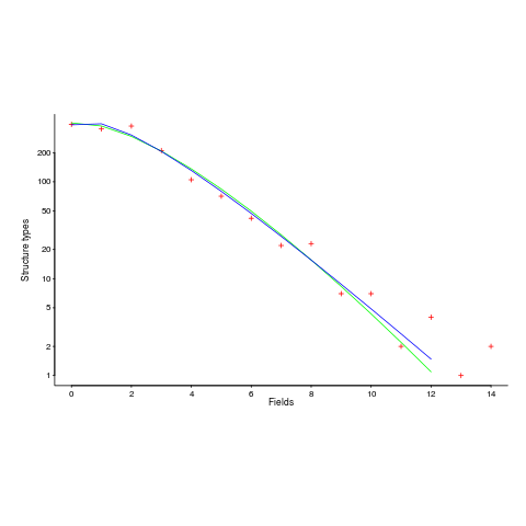
I’m interested in understanding the processes that are generating the data, and having two distributions do such a reasonable job of fitting the data has given me more possible distinct explanations for what is going on than I wanted (if I were interested in prediction, then either distribution looks like it would do a good-enough job).
What are the characteristics of the processes that generate data having each of the distributions?
- A Negative binomial can be viewed as a combination of Poisson distributions (the combination having a Gamma distribution). We could create a story around multiple processes being responsible for the pattern seen, with each of these processes having the impact of a Poisson distribution. Sounds plausible.
- A COM-Poisson distribution can be viewed as a Poisson distribution which is length dependent. We could create a story around the probability of a field being added to a structure type being dependent on the number of existing fields it contains. Sounds plausible (it’s a slightly different idea from preferential attachment).
When fitting a distribution to data, I usually go with the ‘brand-name’ distributions (i.e., the one with most name recognition, provided it matches well enough; brand names are an easier sell then the less well known names).
The Negative binomial distribution is the brand-name here. I had not heard of the COM-Poisson distribution until nine-months ago.
Perhaps the authors of the Racket analysis paper will come up with a theory that prefers one of these distributions, or even suggests another one.
Readers of my evidence-based software engineering book need to be aware of my brand-name preference in some of the data fitting that occurs.
Benford’s law and numeric literals in source code
Benford’s law applies to values derived from a surprising number of natural and man-made processes. I was very optimistic that it would also apply to numeric literals in source code. Measurements of C source showed that I was wrong (the chi-square fit was 1,680 for decimal integer literals and 132,398 for floating literals).
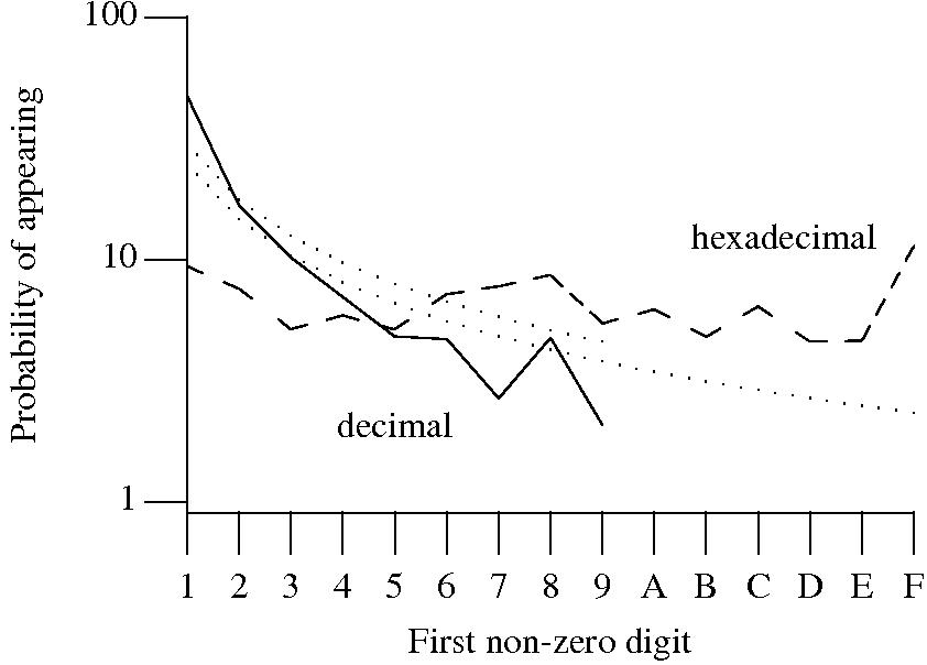
Probability that the leading digit of an (decimal or hexadecimal) integer literal has a particular value (dotted lines predicted by Benford’s law).
What are the conditions necessary for a sample of values to follow Benford’s law? A number of circumstances have been found to result in sample values having a leading digit that follows Benford’s law, including:
Samples that have been found to follow Benford’s law include lists of physical constants and accounting data (so much so that it has been used to detect accounting fraud). However, the number of data-sets containing values whose leading digit follows Benford’s law is not a great as some would make us believe.
Why don’t the leading digits of numeric literals in source code follow Benford’s law?
++/-- operators reduces the number of instances of 1 to increment/decrement a value). But this only applies to integer types, not floating types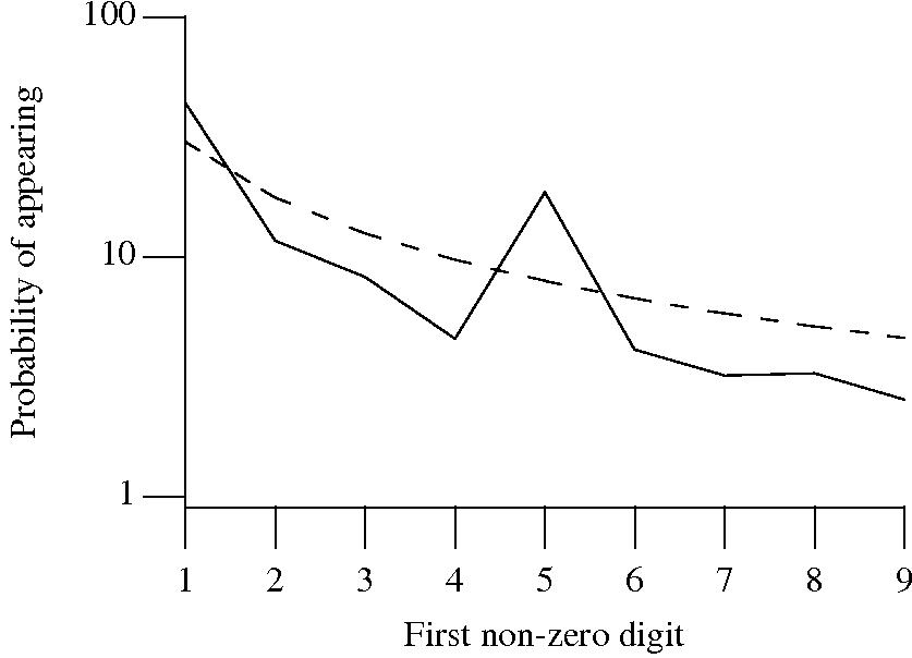
Probability that the leading, first non-zero, digit of a floating literal has a particular value (dashed line predicted by Benford’s law).
5 for the floating-point literals? Have values been rounded to produce 0.5? This looks like an area where methods used for accounting fraud detection might be applied (not that any fraud is implied, just irregularity).These surprising measurements show that there is a lot to the shape of numeric literals that is yet to be discovered.
Recent Comments