Archive
Waiting times and the task selection process
When working on a project, what process do developers use to select the next task to implement?
One way to answer this question is to ask the developers/managers working on the project. However, these people are not always available, and sometimes the actual process used is not what management say it is.
Analysis of the amount of time a task spends in the queue finds various patterns. A previous post discussed some of the theory and data on the distribution of queue task waiting times.
What can be deduced about the task selection process from data on the time they spend in the queue?
From the theoretical perspective there are three task selection processes:
- select the task with the highest priority. The priority of a task might be set by its age (e.g., FIFO, a first, in first out queue), its value to the business, dependency of other tasks, etc.
The distribution of the number of tasks having a given waiting time on some priority queues is a power law (in a FIFO queue the waiting time distribution depends on the distribution of arrival times of new tasks), i.e.,
 , where
  is some constant
 - select a task at random. Random selection comes in various guises including: developers picking what looks to be the most interesting task on the day, or managers deciding that particular functionality would look good during a marketing/sales pitch in a few days.
The distribution of the number of tasks having a given waiting when tasks are selected at random from the queue is an exponential, i.e.,
 , where
  is some constant,
 - select a fraction,
 , of tasks by highest priority, and select the other fraction,
  , of tasks at random.
The distribution of the number of tasks having a given waiting when tasks in this process are a combination of power law and exponential, i.e.,
 , where and are constants.
The average amount of time a task spends in a queue is given by Little’s law, and is independent of the selection process (high priority tasks have a shorter waiting time than low priority tasks, but the overall average is unchanged), i.e., assuming that the averages, and variance, do not change over time, then: (waiting time) equals (average number of tasks in the queue) divided by (average number of tasks implemented per unit of time).
If analysis of the data finds just a power law, then the selection process involves a power law, just an exponential, then some random process(es), and if a combination distributions then a combination of selection processes.
Can anything be learned from knowing the value of or ?
The analysis of various priority+random models finds that, given enough running time, converges to specific values between 1 and 2. Is waiting time data on, say, 1,000 tasks (with an average of 4-hours per task, this is 2-person years) sufficient running time to converge to a good enough approximation of ?
This question can be answered by simulating task queue waiting times. The plot below shows, for 100 projects, the values of fitted to the power law component of the waiting time distribution of projects each having 1,000 tasks (the queue length was fixed at 10 tasks, five task priorities, with  fraction of tasks selected by priority, and the rest randomly; code):
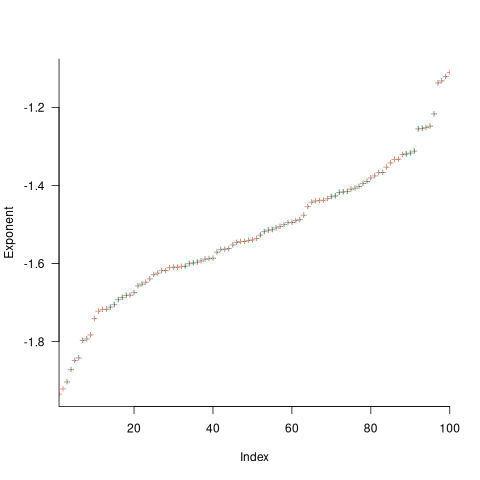
The wide range of fitted exponent values for clearly shows that 1,000 tasks is not sufficient for convergence to a good enough approximation. In fact over 100,000 tasks are needed before exponent values converge within one decimal place.
Similar results are obtained for queue lengths between 5 and 20 tasks, and priority ranges between 3 and 10. Reducing the value of down to 0.7 had a large impact on the tail of the distribution. I have not tried variable length queues.
Sometimes task priorities are changed. One study found that around 8% of bug priorities were changed before the bug was fixed. Simulation found that, when task priorities are changed (at the rate ), rather than randomly selecting a task, the waiting time distribution was a power law (also the long wait time distribution was power law like; code).
Tasks that have spent a long time in the queue are likely to have their priority increased, or be removed from the queue.
If the amount of time spent in the queue contributes some amount of priority to the original task, then the waiting time distribution is exponential (technically it is geometric, the discrete form of exponential; code). The LLM maths assistants did not find any viable equations.
To summarise: The distribution of tasks having a given waiting time has a high variance, which significantly reduces its usefulness for deducing information about the task selection process.
Percentage of methods containing no reported faults
It is often said, with some evidence, that 80% of reported faults, for a program, occur in 20% of its code. I think this pattern is a consequence of 20% of the code being executed 80% of the time, while many researchers believe that 20% of the source code has characteristics that result in it containing 80% of the coding mistakes.
The 20% figure is commonly measured as a percentage of methods/functions, rather than a percentage of lines of code.
This post investigates the expected fraction of a program’s methods that remain fault report free, based on two probability models.
Both models assume that coding mistakes are uniformly scattered throughout the code (i.e., every statement has the same probability of containing a mistake) and that the corresponding coding mistake is contained within a single method (the evidence suggests that this is true for 50% of faults).
A simple model is to assume that when a new fault is reported, the probability that the corresponding coding mistake appears in a particular method is proportional to the method’s length,  in lines of code, of the method. The evidence shows that the distribution of methods containing a given number of lines, , is well-fitted by a power law (for Java:
  ).
).
If  reported faults have been fixed in a program containing
  methods/functions, what is the expected number of methods that have not been modified by the fixing process?
The answer (with help from: mostly Kimi, with occasional help from Deepseek (who don’t have a share chat options), ChatGPT 5, Grok, and some approximations; chat logs) is:
}Li_b(e^{-{F/M}{{zeta(b)}/{zeta(b-1)}}})")
where:  is the Riemann zeta function,
  is the polylogarithm function and
  for Java.
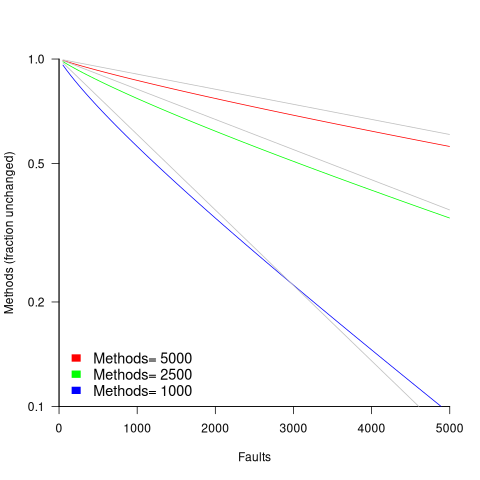
The plot below shows the predicted fraction of unmodified methods against number of faults, for programs of various sizes; the grey lines show the rough approximation:  (code+data):
The observed behavior of most reported faults involving a subset of a program’s methods can be modelled using some form of preferential attachment.
One preferential attachment model specifies that the likelihood of a coding mistake appearing in a method is proportional to ") , where
, where  is the number of previously detected coding mistakes in the method.
The estimated number of unmodified methods is now:
}Li_b(({M zeta(b-1)}/{M zeta(b-1)+a*(F+1) zeta(b)})^{1/a})")
where:  is the average value of
  over all faults (if
  , then
  for a power law with exponent 2.35).
The plot below shows the predicted fraction of unmodified methods against number of faults for a program containing 1,000 methods, for various values of , with the black line showing the fraction of unmodified methods predicted by the simple model above (code+data):
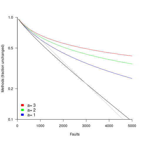
In practice, random selection of the method containing a coding mistake will introduce some fuzziness in the predicted fraction of unmodified methods.
As the number of reported faults grows, the attraction of methods involved in previous reported faults slows the rate at which methods experience their first detected coding mistake.
How realistic are these models?
By focusing on the number of unmodified methods, many complications are avoided.
Both models assume that an unchanging number of methods in a program and that the length of each method is fixed. This assumption holds between each release of a program.
For actively maintained programs, the number of methods in a program changes over time, and the length of some existing methods also changes (if a program were not actively maintained, reported faults would not get fixed).
These models are unlikely to be applicable to programs with short release cycles, where there are few reported faults between releases.
How well do the models’ predictions agree with the data?
At the moment, I am not aware of a dataset containing the appropriate data. Number of faults vs unmodified methods has been added to my list of interesting patterns to notice.
Summary of the derivation of the solutions for the two models.
Simple model
The expected number of unmodified methods, ") , is:
, is:
=sum{L=1}{T}{m_L{P(U_LF)}}") , where
, where  is the length of the longest method,
  is the number of methods of length , and
 ") is the probability that a method of length will be unmodified after fault reports.
is the probability that a method of length will be unmodified after fault reports.
The evidence shows that the distribution of methods containing a given number of lines, , is well-fitted by a power law (for Java: ).
Given a program containing methods, the number of methods of length is:
 , where for Java.
If is large and  , then the sum can be approximated by the Riemann zeta function, , giving:
}}")
The probability that a method containing lines will not be modified by a fault report (assuming that fixing the mistake only involves one method) is:  , where
  is the total lines of code in the program, and the probability of this method not being modified after fault reports is approximately:
^F approx e^{{-F*L}/{P_t}}")
The expected number of empty boxes is:
}}*e^{{-F*L}/{P_t}}}=M/{zeta(b)}Li_b(e^{-F/{P_t}})")
The number of lines of code in a program containing methods is:
}}}=M/{zeta(b)}sum{L=1}{T}{L^{1-b}}=M{{zeta(b-1)}/{zeta(b)}}")
Finally giving:
}Li_b(e^{-{F/M}{{zeta(b)}/{zeta(b-1)}}})")
where is the polylogarithm function.
This equation is roughly, for the purposes of understanding the effect of each variable:

Preferential attachment model
When a mistake is corrected in a method, the attraction weight of that method increases (alternatively, the attraction weight of the other methods decreases). The probability that a method is not modified after fault reports is now:
}=prod{k=0}{F}{{P_t+a*k-L}/{P_t+a*k}}={Gamma({P_t}/a)Gamma({P_t-L}/a+F+1)}/{Gamma({P_t-L}/a)Gamma(P_t/a+F+1)}")
where:  the average value of over all faults, and
  is the gamma function.
applying the Stirling/Gamma–ratio rule, i.e., }/{Gamma(z+b)} approx z^{a-b}") we get:
we get:
})^{F/a} = ((P_t/{P_t+a*(F+1)})^{1/a})^F")
where the expression ^{1/a})^F") is the preferential attachment version of the expression
is the preferential attachment version of the expression ^F") appearing in the simple model derivation. Using this preferential attachment expression in the analysis of the simple model, we get:
appearing in the simple model derivation. Using this preferential attachment expression in the analysis of the simple model, we get:
I don’t have a rough approximation for this expression.
Christmas books for 2024
My rate of book reading has picked up significantly this year. The following are the really interesting books I read, as is usually the case, most were not published in this year.
I have enjoyed Grayson Perry’s TV programs on the art world, so I bought his book “Playing to the Gallery: Helping Contemporary Art in its Struggle to Be Understood“. It’s a fun, mischievous look at the art world by somebody working as a traditional artist, in the sense of creating work that they believe means/says something, rather than works that are only considered art because they are displayed in an art gallery.
“The Computer from Pascal to von Neumann” by H. H. Goldstine. This history of computing from the mid-1600s (the time of Blaise Pascal) to the mid-1900s (von Neumann died in 1957) told by a mathematician who was first involved in calculating artillery firing tables during World War II, and then worked with early computers and von Neumann. This book is full of insights that only a technical person could provide and is a joy to read.
I saw a poster advertising a guided tour of the trees in my local park, organized by Trees for Cities. It was a very interesting lunchtime; I had not appreciated how many different trees were growing there, including three different kinds of Oak tree. Trees for Cities run events all over the UK, and abroad. Of course, I had to buy some books to improve my tree recognition skills. I found “Collins tree guide” by O. Johnson and D. More to be the most useful and full of information. Various organizations have created maps of trees in cities around the world. The London Tree Map shows the location and species information for over 880,000 of trees growing on streets (not parks), New York also has a map. For a general analysis of patterns of tree growth, see “How to Read a Tree” by T. Gooley.
“Medieval Horizons: Why the Middle Ages Matter” by I. Mortimer. This book takes the reader through the social, cultural and economic changes that happened in England during the Middle Ages, which the author specifies as the period 1000 to 1600. I knew that many people were surfs, but did not know that slaves accounted for around 10% of the population, dropping to zero percent during this period. Changes, at least for the well-off, included moving from living in longhouses to living in what we would call a house, art works moved from two-dimensional representations to life-like images (e.g., renaissance quality), printing enables an explosion of books, non-poor people travelled more, ate better, and individualism started to take-off.
Statistical Consequences of Fat Tails: Real World Preasymptotics, Epistemology, and Applications by N. N. Taleb is a mathematically dense book (while the pdf is in color, I was disappointed that the printed version is black/white; this is the one I read while travelling). This book tells you a lot more than you need to know about the consequences of fat tail distributions. Why might you be interested in the problems of fat tails? Taleb starts by showing how little noise it takes for the comforting assumptions implied by the Normal/Gaussian distribution to fly out the window. The primary comforting assumptions are that the mean and variance of a small sample are representative of the larger population. A world of fat tail distributions is one where the unexpected is to be expected, where a single event can wipe out an organization or industry (banks are said to have lost more in the 2008 financial crisis than they had made in the previous many decades). This book is hard going, and I kept at it to get a feel for the answers to some of the objections to the bad news conveyed. There are a couple of places where I should have been more circumspect in my Evidence-based software engineering book.
I have previously reviewed General Relativity: The Theoretical Minimum by Susskind and Cabannes.
“Embracing Defeat: Japan in the Wake of World War II” by John W. Dower describes in harrowing detail the dire circumstances of the population of Japan immediately after World War II and what they had to endure to survive.
For more detailed book reviews, see: Mr. and Mrs. Psmith’s Bookshelf with some excellent and insightful long book reviews, and the annual Astral Codex Ten book review contest usually has a few excellent reviews/books.
For those of you who think that civilization is about to collapse, or at least like talking about the possibility, a reading list. At the practical level, I think sword fighting and archery skills are more likely to be useful in the longer term.
Frequency of non-linear relationships in software engineering data
Causality is an integral part of the developer mindset, and correlation is a common hammer that developers use for the analysis of data (usually the Pearson correlation coefficient).
The problem with using Pearson correlation to analyse software engineering data is that it calculates a measure of linear relationships, and software data is often non-linear. Using a more powerful technique would not only enable any non-linearity to be handled, it would also extract more information, e.g., regression analysis.
My impression is that power laws and exponential relationships abound in software engineering data, but exactly how common are they (and let’s not forget polynomial relationships, e.g., quadratics)?
I claim that my Evidence-based Software Engineering analyses all the publicly available software engineering data. How often do non-linear relationships occur in this data?
The data is invariably plotted, and often a regression model is fitted. A search of the data analysis code (written in R) located 996 calls to plot and 446 calls to glm (used to fit a regression model; shell script).
In calls to plot, the log argument can be used to specify that a log-scale be used for a given axis. When the data has an exponential distribution, I specified the appropriate axis to be log-scaled (18% of cases); for a power law, both axis were log-scaled (11% of cases).
In calls to glm, one or more of the formula variables may be log transformed within the formula. When the data has an exponential distribution, either the left-hand side of the formula is log transformed (20% of cases), or one of the variables on the right-hand side (9% of cases, giving 29% in total); for a power law both sides of the formula are log transformed (12% of cases).
Within a glm formula, variables can be raised to a power by enclosing the expression in the I function (the ^ operator has a special meaning within a formula, but its usual meaning inside I). The most common operation appearing inside I is ^2, i.e., squaring a value. In the following table, only formula that did not log transform any variable were searched for calls to I.
The analysis code contained 54 calls to the nls function, whose purpose is to fit non-linear regression models.
    plot   log="x"  log="y"       log="xy"
    996      4%       14%            11%

    glm    log(x)   log(y)    log(y) ~ log(x)   I()
446 9% 20% 12% 12% |
Based on these figures (shell script), at least 50% of software engineering data contains non-linear relationships; the values in this table are a lower bound, because variables may have been transformed outside the call to plot or glm.
The at least 50% estimate is based on all software engineering, some corners will have higher/lower likelihood of encountering non-linear data; for instance, estimation data often contains power law relationships.
Task backlog waiting times are power laws
Once it has been agreed to implement new functionality, how long do the associated tasks have to wait in the to-do queue?
An analysis of the SiP task data finds that waiting time has a power law distribution, i.e.,  , where
  is the number of tasks waiting a given amount of time; the LSST:DM Sprint/Story-point/Story has the same distribution. Is this a coincidence, or does task waiting time always have this form?
Queueing theory analyses the properties of systems involving the arrival of tasks, one or more queues, and limited implementation resources.
A basic result of queueing theory is that task waiting time has an exponential distribution, i.e., not a power law. What software task implementation behavior is sufficiently different from basic queueing theory to cause its waiting time to have a power law?
As always, my first line of attack was to find data from other domains, hopefully with an accompanying analysis modelling the behavior. It’s possible that my two samples are just way outside the norm.
Eventually I found an analysis of the letter writing response time of Darwin, Einstein and Freud (my email asking for the data has not yet received a reply). Somebody writes to a famous scientist (the scientist has to be famous enough for people to want to create a collection of their papers and letters), the scientist decides to add this letter to the pile (i.e., queue) of letters to reply to, eventually a reply is written. What is the distribution of waiting times for replies? Yes, it’s a power law, but with an exponent of -1.5, rather than -1.
The change made to the basic queueing model is to assign priorities to tasks, and then choose the task with the highest priority (rather than a random task, or the one that has been waiting the longest). Provided the queue never becomes empty (i.e., there are always waiting tasks), the waiting time is a power law with exponent -1.5; this behavior is independent of queue length and distribution of priorities (simulations confirm this behavior).
However, the exponent for my software data, and other data, is not -1.5, it is -1. A 2008 paper by Albert-László Barabási (detailed analysis) showed how a modification to the task selection process produces the desired exponent of -1. Each of the tasks currently in the queue is assigned a probability of selection, this probability is proportional to the priority of the corresponding task (i.e., the sum of the priorities/probabilities of all the tasks in the queue is assumed to be constant); task selection is weighted by this probability.
So we have a queueing model whose task waiting time is a power law with an exponent of -1. How well does this model map to software task selection behavior?
One apparent difference between the queueing model and waiting software tasks is that software tasks are assigned to a small number of priorities (e.g., Critical, Major, Minor), while each task in the model queue has a unique priority (otherwise a tie-break rule would have to be specified). In practice, I think that the developers involved do assign unique priorities to tasks.
Why wouldn’t a developer simply select what they consider to be the highest priority task to work on next?
Perhaps each developer does select what they consider to be the highest priority task, but different developers have different opinions about which task has the highest priority. The priority assigned to a task by different developers will have some probability distribution. If task priority assignment by developers is correlated, then the behavior is effectively the same as the queueing model, i.e., the probability component is supplied by different developers having different opinions and the correlation provides a clustering of priorities assigned to each task (i.e., not a uniform distribution).
If this mapping is correct, the task waiting time for a system implemented by one developer should have a power law exponent of -1.5, just like letter writing data.
The number of sprints that a story is assigned to, before being completely implemented, is a power law whose exponent varies around -3. An explanation of this behavior based on priority queues looks possible; we shall see…
The queueing models discussed above are a subset of the field known as bursty dynamics; see the review paper Bursty Human Dynamics for human behavior related aspects.
Update
A later post walking back some of the claims in this post.
Where are we with models of human learning?
Learning is an integral part of writing software. What have psychologists figured out about the characteristics of human learning?
A study of memory, published in 1885, kicked off the start of modern psychology research. At the start of the 1900s, learning research was still closely tied to the study of the characteristics of what we now call working memory, e.g., measuring the time taken for subjects to correctly recall sequences of digits, nonsense syllables, words and prose. By the 1930s, learning was a distinct subject in its own right.
What is now known as the power law of learning was first proposed in 1926. Wikipedia is right to use the phrase power law of practice, since it is some measure of practice that appears in the power law of learning equation:  , where: is the time taken to do the task,
 is some measure of practice (such as the number of times the subject has performed the task), and ,
  , and are constants fitted to the data.
For the next 70 years some form of power law did a good job of fitting the learning data produced by researchers. Then in 1997 a paper pointed out that researchers were fitting aggregate data (i.e., one equation fitted to all subject data), and that an exponential equation was a better fit to individual subject response times:  . The power law appeared to be the result of aggregating the exponential response performance of multiple subjects; oops.
What is the situation today, 25 years later? Do the subsystems of our brains produce a power law or exponential improvement in performance, with practice?
The problem with answering this question is that both equations can fit the available data quite well, with one being a technically better fit than the other for different datasets. The big difference between the two equations is in their tails, however, it is costly and time-consuming to obtain enough data to distinguish between them in this region.
When discussing learning in my evidence-based software engineering book, I saw no compelling reason to run counter to the widely cited power law, but I did tell readers about the exponential fit issue.
Studies of learnings have tended to use simple tasks; subjects are usually only available for a short time, and many task repetitions are needed to model the impact of learning. Simple tasks tend to be dominated by one primary activity, which means that subjects can focus their learning on this one activity.
Complicated tasks involve many activities, each potentially providing distinct learning opportunities. Which activities will a subject focus on improving, will the performance on one activity improve faster than others, will the approach chosen for one activity limit the performance on a second activity?
For a complicated task, the change in performance with amount of practice could be a lot more complicated than a single power law/exponential equation, e.g., there may be multiple equations with each associated with one or more activities.
In the previous paragraph, I was careful to say “could be a lot more complicated”. This is because the few datasets of organizational learning show a power law performance improvement, e.g., from 1936 we have the most cited study Factors Affecting the Cost of Airplanes, and the less well known but more interesting Liberty shipbuilding from the 1940s.
If the performance of something involving multiple people performing many distinct activities follows a power law improvement with practice, then the performance of an individual carrying out a complicated task might follow a simple equation; perhaps the combined form of many distinct simple learning activities is a simple equation.
Researchers are now proposing more complicated models of learning, along with fitting them to existing learning datasets.
Which equation should software developers use to model the learning process?
I continue to use a power law. The mathematics tend to be straight-forward, and it often gives an answer that is good enough (because the data fitted contains lots of variance). If it turned out that an exponential would be easier to work with, I would be happy to switch. Unless there is a lot of data in the tail, the difference between power law/exponent is usually not worth worrying about.
There are situations where I have failed to successfully add a learning (power law) component to a model. Was this because there was no learning present, or was the learning not well-fitted by a power law? I don’t know, and I cannot think of an alternative equation that might work, for these cases.
for-loop usage at different nesting levels
When reading code, starting at the first line of a function/method, the probability of the next statement read being a for-loop is around 1.5% (at least in C, I don’t have decent data on other languages). Let’s say you have been reading the code a line at a time, and you are now reading lines nested within various if/while/for statements, you are at nesting depth  . What is the probability of the statement on the next line being a
 for-loop?
Does the probability of encountering a for-loop remain unchanged with nesting depth (i.e., developer habits are not affected by nesting depth), or does it decrease (aren’t developers supposed to using functions/methods rather than nesting; I have never heard anybody suggest that it increases)?
If you think the for-loop use probability is not affected by nesting depth, you are going to argue for the plot on the left (below, showing number of loops whose compound-statement contains appearing in C source at various nesting depths), with the regression model fitting really well after 3-levels of nesting. If you think the probability decreases with nesting depth, you are likely to argue for the plot on the right, with the model fitting really well down to around 10-levels of nesting (code+data).
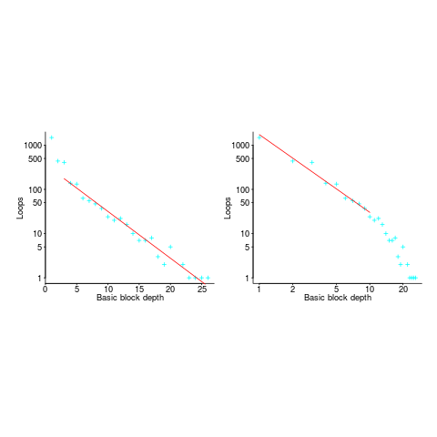
Both plots use the same data, but different scales are used for the x-axis.
If probability of use is independent of nesting depth, an exponential equation should fit the data (i.e., the left plot), decreasing probability is supported by a power-law (i.e, the right plot; plus other forms of equation, but let’s keep things simple).
The two cases are very wrong over different ranges of the data. What is your explanation for reality failing to follow your beliefs in for-loop occurrence probability?
Is the mismatch between belief and reality caused by the small size of the data set (a few million lines were measured, which was once considered to be a lot), or perhaps your beliefs are based on other languages which will behave as claimed (appropriate measurements on other languages most welcome).
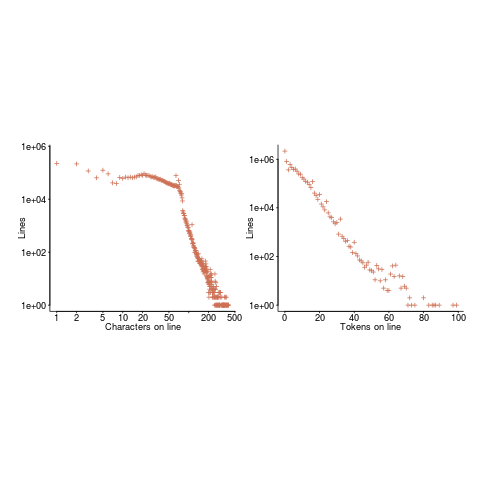
The nesting depth dependent use probability plot shows a sudden change in the rate of decrease in for-loop probability; perhaps this is caused by the maximum number of characters that can appear on a typical editor line (within a window). The left plot (below) shows the number of lines (of C source) containing a given number of characters; the right plot counts tokens per line and the length effect is much less pronounced (perhaps developers use shorter identifiers in nested code). Note: different scales used for the x-axis (code+data).
I don’t have any believable ideas for why the exponential fit only works if the first few nesting depths are ignored. What could be so special about early nesting depths?
What about fitting the data with other equations?
A bi-exponential springs to mind, with one exponential driven by application requirements and the other by algorithm selection; but reality is not on-board with this idea.
Ideas, suggestions, and data for other languages, most welcome.
Developers do not remember what code they have written
The size distribution of software components used in building many programs appears to follow a power law. Some researchers have and continue to do little more than fit a straight line to their measurements, while those that have proposed a process driving the behavior (e.g., information content) continue to rely on plenty of arm waving.
I have a very simple, and surprising, explanation for component size distribution following power law-like behavior; when writing new code developers ignore the surrounding context. To be a little more mathematical, I believe code written by developers has the following two statistical properties:
- nesting invariance. That is, the statistical characteristics of code sequences does not depend on how deeply nested the sequence is within
if/for/while/switchstatements, - independent of what went immediately before. That is the choice of what statement a developer writes next does not depend on the statements that precede it (alternatively there is no short range correlation).
Measurements of C source show that these two properties hold for some constructs in some circumstances (the measurements were originally made to serve a different purpose) and I have yet to see instances that significantly deviate from these properties.
How does writing code following these two properties generate a power law? The answer comes from the paper Power Laws for Monkeys Typing Randomly: The Case of Unequal Probabilities which proves that Zipf’s law like behavior (e.g., the frequency of any word used by some author is inversely proportional to its rank) would occur if the author were a monkey randomly typing on a keyboard.
To a good approximation every non-comment/blank line in a function body contains a single statement and statements do not often span multiple lines. We can view a function definition as being a sequence of statement kinds (e.g., each kind could be if/for/while/switch/assignment statement or an end-of-function terminator). The number of lines of code in a function is closely approximated by the length of this sequence.
The two statistical properties listed above allow us to treat the selection of which statement kind to write next in a function as mathematically equivalent to a monkey randomly typing on a keyboard. I am not suggesting that developers actually select statements at random, rather that the set of higher level requirements being turned into code are sufficiently different from each other that developers can and do write code having the properties listed.
Switching our unit of measurement from lines of code to number of tokens does not change much. Every statement has a few common forms that occur most of the time (e.g., most function calls contain no parameters and most assignment statements assign a scalar variable to another scalar variable) and there is a strong correlation between lines of code and token count.
What about object-oriented code, do developers follow the same pattern of behavior when creating classes? I am not aware of any set of measurements that might help answer this question, but there have been some measurements of Java that have power law-like behavior for some OO features.
A power law artifact
Over the last few years software engineering academics have jumped aboard the power-law band-wagon (examples here and here). With few exceptions (one here) these researchers have done little more that plot their data on a log-log graph and shown that a straight line is a good fit for many of the points. What a sorry state of affairs.
Cognitive psychologists have also encountered straight lines in log-log graphs, but they have been in the analysis of data business much longer and are aware that there might be other distributions that are just as straight in the same places.
A very interesting paper, Toward an explanation of the power law artifact: Insights from response surface analysis, shows how averaging data obtained from a variety of sources (example given is the performance of different subjects in a psychology experiment) can produce a power law where none originally existed. The underlying fault could be that data from a non-linear system is being averaged using the arithmetic mean (I suspect that I have done this in the past), which it turns out should only be used to average data from a linear system. The authors list the appropriate averaging formula that should be used for various non-linear systems.
Recent Comments