Archive
Maximum Adds per second for 1950s/early 1960s computers
Relative digital computer performance has been measured, since the mid-1960s, by timing how long it takes to execute one or more programs. Until the early 1990s Whetstone was widely used, and then SPEC brought things up to date.
Running the same program on multiple computers requires that it be written in a language that is available on those computers. Fortran, Cobol and Algol 60 started to spread at the start of the 1960s (there were 21 Algol 60 compilers were available in 1961), but it took a while for old habits to change, and for specific programs to be accepted as reasonable benchmarks.
One early performance comparison method involved calculating a sum of instruction timings, weighted by instruction frequency. The view of computers as calculating machines meant that the arithmetic instructions add/multiply/divide were often the focus of attention.
A calculation based on instructions assumes that timings do not vary with the value of the operand (which multiple and divide often do, and addition sometimes does), that instruction time can be measured independent of the time taken to load the values from memory (which is not possible for when one operand is always loaded from memory), and instruction frequency is representative of typical applications.
With regard to instruction timings, some manufacturers quoted an average, while others gave a range of values. One publication quotes arithmetic timings for specific numeric values. The “Data Processing Equipment Encyclopedia: Electronic Devices”, published in 1961 by Gille Associates, lists the characteristics of 104 computers, including the time taken to perform the arithmetic operations: addition 555555+555555, multiplication 555555*555555, and division 308641358025/555555. The results were mostly for fixed point, sometimes floating-point, or both, and once in double precision. In practice small numeric values dominate program execution. I suspect the publishers picked large values because customers think of computers as working on big/complicated problems.
The time taken to load a value from memory can be a significant percentage of execution time, which is why processor cache has such a big impact on performance. In the 1950s main memory was often the cache, with the rest of memory held on a rotating drum. Hardware specifications often gave arithmetic instruction timings for both excluded and included memory access cases.
The plot below shows the execution time of the Add instruction excluding/including memory access on the same computer for pre-1961 computers, with regression line of the form:  (grey line shows
  ; code+data):
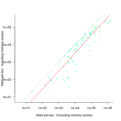
When memory access time is included in the Add instruction timing, the maximum rate of instructions per second decreases by approximately a factor of four, compared to when memory access time is excluded.
What was the frequency distribution of instructions executed by computers in the 1950s/1960s? I suspect it was a simplified form of today’s frequency distribution. Simplified in the sense of there being fewer variants of commonly used instructions and way fewer addressing modes.
Application domains were divided into scientific/engineering and commercial. One executed lots of float-point instructions, the other executed none. One did a lot of reading/writing of punched cards/magnetic tape, the other did hardly any. If we want to compare early the performance of cpus across the decades, methods that assume a significant amount of I/O have to be ignored, or the I/O component reverse engineered out.
Kenneth Knight, in his PhD thesis (no copy online), published the most detailed and extensive analysis, and data. Knight included an I/O component in his performance formula, but this was relatively small for scientific/engineering.
The table below lists the instruction weights for scientific/engineering applications published by Knight and Arbuckle, a Manager of Product Marketing at IBM:
Instruction or Operation Knight Arbuckle Floating Point Add/Sub 10% 9.5% Floating Point Multiply 6% 5.6% Floating Point Divide 2% 2.0% Fixed add/sub 10% Load/Store 28.5% Indexing 22.5% Conditional Branch 13.2% Miscellaneous 72% 18.7% |
Solomon published weights for the IBM 360 family. By focusing on a range of compatible computers the evaluation was not restricted to generic operations, and used timings from 60 different instructions.
The following analysis is based on data extracted from the 1955, 1961, and 1964 (which does not have a handy table of arithmetic instruction timings; thanks to Ed Thelen for converting the scanned images) surveys of domestic electronic digital computing systems published by the Ballistic Research Laboratory.
If the performance of computers from the 1950s/1960s is to be compared with performance in later decades, which computers from the 1950s/1960s should be included? Of the 228 computers listed in a January 1964 survey of the roughly 14k+ computing systems manufactured or operational, over 50% are bespoke, i.e., they are unique. The top 10 systems represent over 75% of manufactured systems; see table below (the IBM 604 was an electronic calculating punch, and is not listed):
   Quantity   SYSTEM           Cumulative percentage
   5,000+      IBM 1401                  36%
   2,500+      IBM 650                   54%
     693       IBM CPC                   59%
     490       LGP 30                    63%
     478       BURROUGHS B26O/B270/B280  66%
     400+      LIBRATROL 500             69%
     300+      BENDIX G-15               71%
     300       CONTROL DATA 160A         73%
     267       IBM 607                   75%
210 BURROUGHS E103/E101 77% |
When programming in machine code, developers put a lot of effort into keeping frequently used values in registers (developers can still sometimes do a better job than compilers), and overlapping memory access with other operations. The plot below shows the maximum number of add and multiply instructions per second that could be executed without accessing storage (code+data):
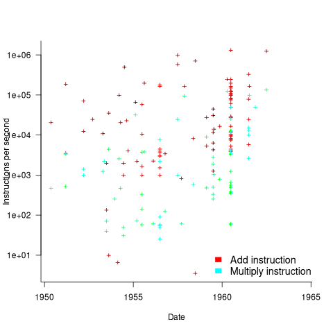
The systems capably of less than ten instructions per second are essentially early desktop calculators.
What percentage of Add instructions accessed memory? As far as I can tell, none of the performance comparison reports/papers address with this question. To be continued…
Relative performance of computers since the 1990s
What was the range of performance of desktop’ish computers introduced since the 1990s, and what was the annual rate of performance increase (answers for earlier computers)?
Microcomputers based on Intel’s x86 family was decimating most non-niche cpu families by the early 1990s. During this cpu transition a shift to a new benchmark suite followed a few years behind. The SPEC cpu benchmark originated in 1989, followed by a 1992 update, with the 1995 update becoming widely used. Pre-1995 results don’t appear on the SPEC website: “Because SPEC’s processes were paper-based and not electronic back when SPEC CPU 92 was the current benchmark, SPEC does not have any electronic storage of these benchmark results.” Thanks to various groups, some SPEC89/92 results are still available.
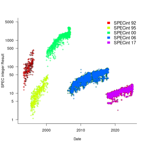
The following analysis uses the results from the SPEC integer benchmarks, which was changed in 1992, 1995, 2000, 2008, and 2017.
Every time a benchmark is changed, the reported results for the same computer change, perhaps by a lot. The plot below shows the results for each version of the benchmark (code+data):
Provide a few conditions are met, it is possible to normalise each set of results, allowing comparisons to be made across benchmark changes. First, results from running, say, both SPEC92 and SPEC95 on some set of computer needs to be available. These paired results can be used to build a model that maps result values from one benchmark to the other. The accuracy of the mapping will depend on there being a consistent pattern of change, i.e., a strong correlation between benchmark results.
The plot below shows the normalised results, along with regression models fitted to each release (code+data):
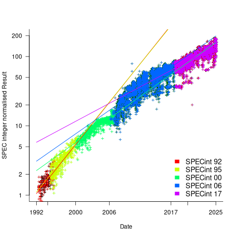
What happened around 2007? Dennard scaling stopped, and there is an obvious meeting of two curves as one epoch transitioned into another. Since 2007 performance improvements have been driven by faster memory, larger caches, and for some applications multiple on-die cpus.
The table below shows the annual growth in SPECint performance for each of the benchmark start years, over their lifetime.
      Year   Annual growth
      1992       26.2%
      1995       25.9%
      2000       14.2%
      2007       13.9%
2017 10.5% |
In 2025, the cpu integer performance of the average desktop system is over 100 times faster than the average 1992 desktop system. With the first factor of 10 improvement in the first 10 years, and the second factor of 10 in the previous 20 years.
Early research on economies of scale for computer systems
Before microprocessor cost/performance wiped out (in the early 1990s) other cpu platforms (e.g., mainframes and minis), people argued that computer hardware benefited from economies of scale.
The claimed benefit was more bang for the buck, i.e., more compute for less money.
Checking this claim requires treating pre-microprocessor computer systems and the later microprocessor-based systems as two separate cases, because many of the factors driving costs and performance are very different.
Today’s large microprocessor-based computer systems achieve economies of scale through discounts from bulk purchases and spreading fixed costs across multiple systems. The data is available, and the economic analysis is straight forward.
A lack of reliable data on the costs of designing/building pre-microprocessor computer systems rules out an economic analysis of cost/performance from first principles. The data that was/is available is the cost of computer systems and some indicators of performance (such as instruction timings or benchmarks).
Now, the observed fact that the cost of compute was decreasing over time is unrelated to the claim that the cost of compute decreases as the size of the computer increases.
Assuming a power law relationship between computer cost,  , and size,
  , at a point in time, we have:
  , where
  is some constant. Economies of scale occur when:
In his detailed cost/performance analysis of computers between 1944-1967, Kenneth Knight treated computers launched in the same year as effectively occurring at the same time. He also built a single model, with year included as an explanatory variable, which means the fitted rate of decrease is the same over all years (rather than varying between years).
The plot below uses Knight’s 1953-1961 data, and shows operations per second against seconds per dollar (a confusing combination, but what Knight used), with fitted regression lines for three years using Knight’s model (code and data)
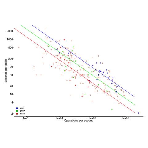
The fitted exponent for this form of x/y axis maps to a value which has , i.e., there are economies of scale.
It so happens that the value of the Knight’s fitted exponent is close to that proposed in a 1953 paper (“High speed arithmetic: The digital computer as a research tool”, no online copy):
It used to cost one cent to do a multiplication on a desk calculator; now it is more like four cents; but with these big machines we can do a million in an hour for $400, and that means twenty-five multiplications for a cent! I believe that there is a fundamental rule, which I modestly call Grosch's law, giving added economy only as the square root of the increase in speed-that is, to do a calculation ten times as cheaply you must do it one hundred times as fast. |
which did indeed become widely known as Grosch’s law.
Having been given a lucky kick-start by Knight (fitted individually, years are not close to Grosch’s law), checking for agreement with Grosch’s law became a focus for later studies. While various papers highlighted problems with the later data analysis (e.g., the regression techniques and sample noise producing mathematical artifacts), Grosch’s law ceased being a thing because mainframes/minicomputers ceased being a thing.
Did mainframe/mincomputers have economies of scale in the years after Knight’s data? It’s difficult to tell, the publicly available data is too sparse to support reliable analysis.
CPU frequency not relevant to SPEC benchmark performance
Despite the end of Dennard scaling around 2005-7 computer performance, as measured by the SPEC cpu benchmarks, continues to improve. What is driving this ongoing increase in performance, given that cpu clock rates have stopped increasing?
The plot below shows 9,161 results from the SPEC CPU integer benchmark, plus the fitted regression line  (code+data):
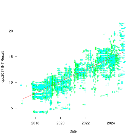
There is a scattering of benchmark results because manufacturers offer systems having a range of performance.
Possible factors driving the ongoing increases in system performance include increased DRAM-memory bandwidth, and cpu improvements such as larger caches and more accurate branch prediction. While Moore’s law (i.e., rate of growth of the number of transistors on a chip) has slowed down a lot, the number of transistors in a processor chip has continued to increase (many of these transistors have been used to build chips that contain multiple cpu cores).
The SPEC benchmark result data includes a lot of information about the system that ran the benchmarks, including: processor family/model, number of cpu cores, clock frequency, amount of memory installed and its type.
Results from SPEC CPU2017, the current version of the benchmark, are available from the start of 2017 to now. The following analysis uses these results. Results from the SPEC CPU2006 benchmark are also available, and a regression model fitted to the results from the 780 systems that ran both benchmarks, gives the mapping from CPU INT 2006 to CPU INT 2017 as:  .
.
The processor information in the results file usually specifies family name plus model number/name. The model information usually correlates with clock frequency, perhaps cache size, or gpu support; some examples below.
    AMD EPYC 4464P                AMD EPYC 4564P
    AMD Ryzen 9 7950X             AMD Ryzen 7 5800X
    Intel Xeon Platinum 8490H     Intel Xeon Gold 6438N
Intel Xeon E3-1220 v3 Intel Xeon E5-2697 v3 |
The family name is sufficient for an initial analysis. Details of any cache size differences between models can always be included in a later analysis. The following table shows the number of processor x86 based families present in the 2017 INT results (total 9,161):
           AMD EPYC           AMD Ryzen               Intel
               1475                   7                   1
      Intel Celeron       Intel Core i3       Intel Core i5
                 16                  31                   2
      Intel Core i7       Intel Pentium          Intel Xeon
                  1                  30                 605
  Intel Xeon Bronze        Intel Xeon D       Intel Xeon E3
                167                  12                  16
      Intel Xeon E5       Intel Xeon E7     Intel Xeon Gold
                  3                   2                3994
Intel Xeon Platinum   Intel Xeon Silver        Intel Xeon W
1822 969 8 |
The memory information usually includes total bytes, number of memory sticks and interface standard (e.g., DDR2/3/4/5); some examples below.
    64 GB (2 x 32 GB 2Rx4 PC5-5600B-R, running at 5200)
    64 GB (2 x 32 GB 2Rx8 PC4-3200AA-E)
    256 GB (8*1GB DDR2-400 DIMMS per 4 core module)
    192 GB (4 x 12 x 4 GB DDR3-1333R, ECC, CL9)
    32 GB (8 x 4 GB Dual-rank PC2-6400 CL5-5-5 FB-DIMMs)
24 GB (6 x 4 GB DDR3-1333 downclocked to 1066 MHz) |
The memory bandwidth can be calculated from the interface standard used. The names of modern DRAM interface standards start with either DDR or PC, and a number, a hyphen and then another number. The values appearing in the SPEC results don’t always follow the naming rules listed in the standard (e.g., last number of a PC name using the corresponding DDR number), and in a few cases a digit was dropped from the last number. Where possible the ‘obvious’ edits were made (sometimes values were just wrong), see code for details. The following table shows the number of interface standards represented in the 2017 CPU INT results (total 9,161; in the 2006 results DDR names predominated):
PC4-2400  PC4-2666  PC4-2933  PC4-3200  PC4-4800 PC5-11200 PC5-12800
      26      2248      2163      2080         6         2         3
PC5-4800  PC5-5200  PC5-5600  PC5-6400     PC5-8  PC5-8800
1735 5 653 233 2 5 |
Once the memory is identified, its bandwidth can be looked up (bespoke memory stick clock rates were ignored). Fitting a regression model to the data, with the CPU INT (cpu integer benchmark) result as the outcome, we get (using a multiplicative model allows each factor to have a percentage impact; code+data):

where:  is the memory bandwidth in megabytes per second,
  is cpu frequency in MHz, and
  is the fitted constant for each processor family.
The cpu frequency varies between 1.7 and 4.7 GHz (a ratio of 1:2.8), the memory bandwidth between 19,200 and 51,200 MB/s (a ratio of 1:2.7), and processor family performance impact ratio was 1:2.2. Given the fitted power laws, this range of cpu frequencies could impact performance by around 22%, while the range of memory bandwidth could impact performance by a factor of two.
This fitted model implies that cpu frequency changes, over the range supported by systems since 2017, have almost no impact on the performance of integer-based programs, i.e., no floating point.
I thought there might be a correlation between memory bandwidth and cpu frequency (because vendors would use faster memory in systems with faster cpus). The plot below shows CPU frequency against memory bandwidth (both axis use linear scales), plus a fitted regression line in red (code+data):
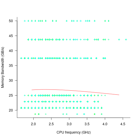
I was wrong. There does not appear to be any connection between a system’s cpu frequency and its memory bandwidth.
These days, most x86 chips include multiple processors, with each processor taking a share of memory bandwidth. Increasing memory bandwidth is essential, if all cores are to be kept busy.
The SPEC CPU benchmark measures the performance of a single processor. If only one of the cpu cores available on a system is being used, that core has the benefit of memory bandwidth that usually has to be shared.
To what extent is a single core benchmark relevant today? I suspect that most programs run on a single core, but developers sometimes attempt to spread cpu intensive programs over multiple cores. As always, data is needed.
The SPEC benchmark is useful for cpu designers (the original target market) and compiler writers wanting to measure the impact of fancy new optimizations.
Memory bandwidth: 1991-2009
The Stream benchmark is a measure of sustained memory bandwidth; the target systems are high performance computers. Sustained in the sense of distance running, rather than a short sprint (the term for this is peak memory bandwidth and occurs when the requested data is in cache), and bandwidth in the sense of bytes of memory read/written per second (implemented using chunks the size of a double precision floating-point type). The dataset contains 1,018 measurements collected between 1991 and 2009.
The dominant characteristic of high performance computing applications is looping over very large arrays, performing floating-point operations on all the elements. A fast floating-point arithmetic unit has to be connected to a memory subsystem that can keep it fed with new floating-point values and write back computed values.
The Stream benchmark, in Fortran and C, defines several arrays, each containing max(1e6, 4*size_of_available_cache) double precision floating-point elements. There are four loops that iterate over every element of the arrays, each loop containing a single statement; see Fortran code in the following table (q is a scalar, array elements are usually 8-bytes, with add/multiply being the floating-point operations):
Name Operation Bytes FLOPS Copy a(i) = b(i) 16 0 Scale a(i) = q*b(i) 16 1 Sum a(i) = b(i) + c(i) 24 1 Triad a(i) = b(i) + q*c(i) 24 2 |
A system’s memory bandwidth will depend on the speed of the DRAM chips, the performance of the devices that transport bytes to the cpu, and the ability of the cpu to handle incoming traffic. The Stream data contains 21 columns, including: the vendor, date, clock rate, number of cpus, kind of memory (i.e., shared/distributed), and the bandwidth in megabytes/sec for each of the operations listed above.
How does the measured memory bandwidth change over time?
For most of the systems, the values for each of Copy, Scale, Sum, and Triad are very similar. That the simplest statement, Copy, is sometimes a bit faster/slower than the most complicated statement, Triad, shows that floating-point performance is much smaller than the time taken to read/write values to memory; the performance difference is random variation.
Several fitted regression models explain over half of the variance in the data, with the influential explanatory variables being: clock speed, date, type of system (i.e., PC/Mac or something much more expensive). The plot below shows MB/sec for the Copy loop, with three fitted regression models (code+data):
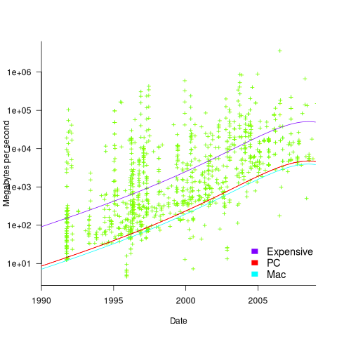
Fitting these models first required fitting a model for cpu clock rate over time; predictions of mean clock rate over time are needed as input to the memory bandwidth model. The three bandwidth models fitted are for PCs (189 systems), Macs (39 systems), and the more expensive systems (785; the five cluster systems were not fitted).
There was a 30% annual increase in memory bandwidth, with the average expensive systems having an order of magnitude greater bandwidth than PCs/Macs.
Clock rates stopped increasing around 2010, but go faster DRAM standards continue to be published. I assume that memory bandwidth continues to increase, but that memory performance is not something that gets written about much. The memory bandwidth on my new system is  MB/sec. This 2024 sample of one is 3.5 times faster than the average 2009 PC bandwidth, which is 100 times faster than the 1991 bandwidth.
The LINPACK benchmarks are the traditional application oriented cpu benchmarks used within the high performance computer community.
Median system cpu clock frequency over last 15 years
We are all familiar with graphs showing the growth of cpu clock frequency over time. The data for these plots is based on vendor announcements listing the characteristics of their latest products, and invariably focuses on the product which is the fastest or contains the most transistors or the lowest power consumption.
Some customers buy the cpu with the highest/most/lowest, but many are happy to pay less for, for good enough. What does a graph of average customer cpu clock frequency over time look like?
Vendors sometimes publish general sales figures, but I have never seen one broken down by clock frequency. However, a few sites collect user system data, including:
- A subset of the Linux Counter project data is available. This does not contain explicit date information, but a must-be-later-than date can be inferred from the listed Linux kernel version,
- Hardware for BSD has data going back to December 2014, but there is no obvious way to extract it (I have not tried that hard),
- the BSDstats project (variable website availability) has been collecting data on machines running some derivative of BSD since August 2008; it contains around 200 times more cpu data than the known Linux Counter data. While the raw data is not available, approximately monthly reports are available on the Wayback Machine.
A BSDstats cpu history was obtained using waybackpack to download the available stored cpu summary pages, followed by html2text, and an awk script to extract the cpu frequency/count data.
BSDstats obtains the cpu information via a call to the sysctl command. For many Intel processors, but not AMD processors, the returned string includes the frequency (to see your cpu information on Linux systems type: more /proc/cpu), for instance:
Celeron(R) CPU 2.80GHz | 336 Pentium(R) 4 CPU 3.00GHz | 258 Pentium(R) 4 CPU 2.40GHz | 170 Athlon(tm) 64 Processor 3000+ | 43 Athlon(tm) 64 X2 Dual Core Processor 4200+ | 28 Athlon(tm) 64 Processor 3500+ | 27 |
For simplicity, only those rows containing frequency information were used in this analysis; 67% of the strings explicitly included a frequency (this saved me having to build a table to map AMD cpu strings to their corresponding frequency).
The plot below shows median cpu frequency (in red), along with the top/bottom 10% cpu frequencies, based on the Wayback Machine’s copy of the webpage on a given date, for a total of 2,304,446 cpu identities (code+data):
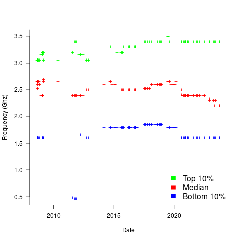
Broadly, the plot shows that cpu frequencies have essentially remained unchanged since 2008, with systems running BSD having a median frequency of 2.5 GHz, with 10% of systems having a frequency over 3.5 GHz, and 10% of systems a frequency below 1.5 GHz.
I was surprised at how many different frequencies were present in the data; often over 50. A look at the large number of different versions of Intel x86 cpus suggests that this is to be expected.
How representative is this sample of BSD systems, compared to the many more systems running Linux and Windows?
This begs the question of what kinds of environments are being compared. Are these desktop systems, local or hosted clusters, cloud systems?
The plot below shows the total number of cpus summarised on each Wayback Machine snapshot (code+data):
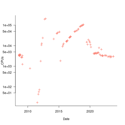
A few thousand systems are likely to be personal desktop systems, while the tens of thousands are likely to be clusters or small cloud providers.
Pointers to more data, particularly pre-2000, most welcome.
Relative performance of computers from the 1950s/60s/70s
What was the range of performance of computers introduced in the 1950, 1960s and 1970s, and what was the annual rate of increase?
People have been measuring computer performance since they were first created, and thanks to the Internet Archive the published results are sometimes available today. The catch is that performance was often measured using different benchmarks. Fortunately, a few benchmarks were run on many systems, and in a few cases different benchmarks were run on the same system.
I have found published data on four distinct system performance estimation models, with each applied to 100+ systems (a total of 1,306 systems, of which 1,111 are unique). There is around a 20% overlap between systems across pairs of models, i.e., multiple models applied to the same system. The plot below shows the reported performance for pairs of estimates for the same system (code+data):

The relative performance relationship between pairs of different estimation models for the same system is linear (on a log scale).
Each of the models aims to produce a result that is representative of typical programs, i.e., be of use to people trying to decide which system to buy.
- Kenneth Knight built a structural model, based on 30 or so system characteristics, such as time to perform various arithmetic operations and I/O time; plugging in the values for a system produced a performance estimate. These characteristics were weighted based on measurements of scientific and commercial applications, to calculate a value that was representative of scientific or commercial operation. The Knight data appears in two magazine articles analysing systems from the 1950s and 1960s (the 310 rows are discussed in an earlier post), and the 1985 paper “A functional and structural measurement of technology”, containing data from the late 1960s and 1970s (120 rows),
- Ein-Dor and Feldmesser also built a structural model, based on the characteristics of 209 systems introduced between 1981 and 1984,
- The November 1980 Datamation article by Edward Lias lists what he called the KOPS (thousands of operations per second, i.e., MIPS for slower systems) value for 237 systems. Similar to the Knight and Ein-dor data, the calculated value is based on weighting various cpu instruction timings
- The Whetstone benchmark is based on running a particular program on a system, and recording its performance; this benchmark was designed to be representative of scientific and engineering applications, i.e., floating-point intensive. The design of this benchmark was the subject of last week’s post. I extracted 504 results from Roy Longbottom’s extensive collection of Whetstone results going back to the mid-1960s.
While the Whetstone benchmark was originally designed as an Algol 60 program that was representative of scientific applications written in Algol, only 5% of the results used this version of the benchmark; 85% of the results used the Fortran version. Fitting a regression model to the data finds that the Fortran version produced higher results than the Algol 60 version (which would encourage vendors to use the Fortran version). To ensure consistency of the Whetstone results, only those using the Fortran benchmark are used in this analysis.
A fifth dataset is the Dhrystone benchmark followed in the footsteps of the Whetstone benchmark, but targetting integer-based applications, i.e., no floating-point. First published in 1984, most of the Dhrystone results apply to more recent systems than the other benchmarks. This code+data contains the 328 results listed by the Performance Database Server.
Sometimes slightly different system names appear in the published results. I used the system names appearing in the Computers Models Database as the definitive names. It is possible that a few misspelled system names remain in the data (the possible impact is not matching systems up across models), please let me know if you spot any.
What is the best statistical technique to use to aggregate results from multiple models into a single relative performance value?
I came up with various possibilities, none of which looked that good, and even posted a question on Cross Validated (no replies yet).
Asking on the Evidence-based software engineering Discord channel produced a helpful reply from Neal Fultz, i.e., use the random effects model: lmer(log(metric) ~ (1|System)+(1|Bench), data=Sall_clean) ; after trying lots of other more complicated approaches, I would probably have eventually gotten around to using this approach.
Does this random effects model produce reliable values?
I don’t have a good idea how to evaluate the fitted model. Looking at pairs of systems where I know which is faster, the relative model values are consistent with what I know.
A csv of the calculated system relative performance values. I have yet to find a reliable way of estimating confidence bounds on these values.
The plot below shows the performance of systems introduced in a given year, on a relative scale, red line is a fitted exponential model (a factor of 5.5 faster, annually; code+data):
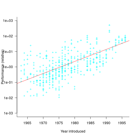
If you know of a more effective way of analysing this data, or any other published data on system benchmarks for these decades, please let me know.
The lifetime of performance coding issues
Coding activities that a developer might spend time on include: adding new functionality, fixing a reported fault, or fiddling with existing code with the intent of making it ‘better’ in some sense (which these days goes by the catch-all name of refactoring).
Improving performance, e.g., changing software to use less cpu/memory is considered, by developers, to make it ‘better’ (whether users are likely to notice the difference, or management see a ROI is for another article). There is a breed of developer whose DNA encodes for pleasure receptors that are only fire when working to reduce the amount of cpu/memory used by a program.
The paper Characterizing the evolution of statically-detectable performance issues of Android Apps by Das, Di Penta, and Malavolta studied the creation/removal of nine distinct performance coding issues in the source of 316 Android Apps (118 Apps contained five or more issues); a total of 2,408 performance issues were tracked.
What patterns might be present in the paper’s performance issues data?
I would expect there to be more creations in Apps containing more code, and more removals the longer an App is maintained; both very obvious. With more developers working on an App, there are going to be more creations and removals; do they cancel out? Management might decide to invest time in performance improvements for the next release, which would cause a spike in the number of removals per unit time.
How long do the nine performance issues survive in code, before being removed? The plot below shows the Kaplan Meier survival curve for Apps containing at least five issues (dotted blue/green are the 95% confidence intervals, code+data):
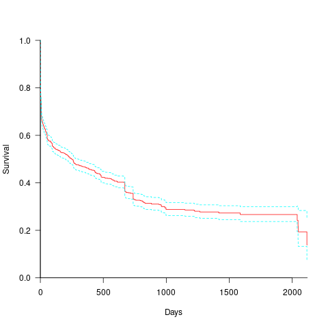
Around 15% of issues were removed on the day they are created, and by the eighth day around 30% had been removed. The roughly steady decline lasts for two-years, followed by almost stasis. Is two-years the active development lifetime of a successful Android App?
In isolation, the slope of the survival curve between eight days and two-years is not that interesting (it could be used to rule out models of the issue discovery process, e.g., happenstance discovery while working on other tasks). However, comparing it against the corresponding survival curve for reported faults tells us something about developer/management investment priorities for the two kinds of tasks, as measured by time to fix (which is a proxy for effort invested).
Unfortunately, this study did not collect information on coding mistake lifetimes, or time between a fault being reported and fixed. There have been studies investigating the survival time of coding mistakes. Reported faults should have the lowest survival rate, while the survival of coding mistakes will depend on the number of users (i.e., more users creates more opportunities to experience a fault and report it).
What factors influence performance issue time-to-fix?
The data includes information on the kind of performance issue, the number of times the App has been downloaded from the Google Play Store, and the number of contributors to the App.
Using these variables, a Cox proportional hazards model was fitted to model the survival time. In a proportional hazards model, the model coefficients are not absolute values, but provide ratio information. For instance, the following table shows the coefficients of the fitted model (code+data). Using these coefficients, we can compare the time taken to fix, say, a FloatMath issue relative to a ViewTag issue. The coefficient ratio  is the estimated ratio of fix times of the two respective issues.
Coefficient Standard error Performance issue FloatMath 0.64445 0.14175 HandlerLeak 0.69958 0.12736 Recycle 0.83041 0.11386 UseSparseArrays 0.73471 0.12493 UseValueOf 0.64263 0.11827 ViewHolder 0.87253 0.14951 ViewTag 5.24257 0.46500 Wakelock 3.34665 0.72014 Downloads 50-100 0.62490 0.26245 100-500 0.64699 0.22494 500-1000 0.56768 0.23505 1000-5000 0.50707 0.22225 5000-10000 0.53432 0.22486 10000-50000 0.62449 0.21626 50000-100000 0.42214 0.23402 100000-500000 0.21479 0.25358 1000000-5000000 0.40593 0.21851 10000000-50000000 0.03474 0.61827 100000000-500000000 0.30693 0.39868 1000000000-5000000000 0.41522 0.61599 NA 0.03868 1.02076 Contributors 1.04996 0.01265 |
There is not a lot of difference in the coefficients for the number of downloads (the model fit is poor when the Standard error is close to the Coefficient value).
The paper Investigating Types and Survivability of Performance Bugs in Mobile Apps analyses a smaller dataset of performance issue lifetimes.
WebAssembly vs JavaScript performance: 2023 edition
WebAssembly is an assembly-like language intended to be executed by web browsers on an internal stack machine. The intent is that compilers for high-level languages (i.e., C, Cobol, and C#) treat WebAssembly just like they would the assembly language of a cpu. Some substantial applications have been ported, e.g., the R statistical environment, which is written in C and Fortran.
Some people claim that WebAssembly based applications will run faster, and consume less power, than those written in JavaScript or PHP. Now, one virtual machine is as much like any other. Performance differences are driven by compiler optimizations, the ease with which particular language features can be mapped to the available instructions, and an application’s use of easy/hard to map high-level language features.
Researchers have run benchmarks to compare the runtime performance and power consumption of Wasm against other browser based languages, and this post analyses the runtime performance results from two papers.
TL;DR: Relative performance for Wasm/JavaScript varies across browsers and programs. Everything interacts with everything else, which makes analysis complicated.
As is the case with most data analysis in software engineering, the researchers used rudimentary statistical techniques (which is a shame given the huge effort that went into collecting the data). The conclusions of both papers is that for WebAssembly/JavaScript, relative performance issues are complicated, but the techniques they used did not enable them to understand why.
What kind of statistical techniques are applicable for analysing these benchmarks?
Use of different languages/browsers might be expected to have some percentage impact on performance, e.g., programs written in language X will be p% faster/slower. The following equation is one modelling approach, and this equation can be fitted using nonlinear regression:
(1+c_j Browser_j)") , where: is a constant,
, where: is a constant,  is the fitted constant for language
  , and
, and  is the fitted constant for browser
The problem with this equation is that it involves a separate equation for each combination of language/browser (assuming that all benchmarks are bundled together in the value of ). It is possible to use a single equation when there are just two languages/two browsers, by mapping them to the values 0/1.
All languages/browsers/benchmarks can be included in a single linear regression model by treating them as factors in a log transformed model; the equation is:  , where:
  is the fitted constant for benchmark
  . The values of , , and are zero, or one for the corresponding fitted constant. All the factors on the right-hand-side are discrete, so a log transform has nothing to distort.
The fitted equation can then be transformed to:

This model assumes that each factor is independent of the others, i.e., the relative performance of each language does not depend on the browser, and that relative performance does not significantly vary between benchmarks, e.g., if  runs 10% faster when implemented in
  , then
  also runs close to 10% faster when implemented in .
How well did the benchmark data from the two papers fit this model, and what were the performance numbers?
The study WebAssembly versus JavaScript: Energy and Runtime Performance by De Macedo, Abreu, Pereira, and Saraiva ran a wide range of benchmarks. It compared C/Wasm/JavaScript running on Chrome/Firefox/Edge. One set of benchmarks were 10 small compute-intensive programs (in Wasm/JavaScript), which were executed with small/medium/large amounts of input data; the other set of benchmarks were two large applications WasmBoy is a Game-boy/Gameboy Color Emulator (written in Typescript and compiled to Wasm), and PSPDFKit supporting viewing, annotating, and filling in forms in PDF documents (written in C/C++ and compiled to a both a subset of JavaScript and Wasm).
Results from the 10 small benchmarks showed strong interactions between browser and language (i.e., Wasm performance relative to JavaScript, varied between browsers; with Edge being faster and Firefox being slower), and a lot of interaction between benchmark and input data size. Support for Wasm is relatively new, relative to the much more mature JavaScript, so it’s not surprising that different browsers have different performance; I’m arm waving when I say that the input size dependency may be related to JIT issues (code).
When interactions are included, the fitted equation has the form:

Analysing the results for the two applications, we find that:
- WasmBoy: the factors were independent, and WebAssembly was faster than JavaScript. The
 factor was 0.84 for Wasm and 1 for JavaScript,
 - PSPDFKit: there was interaction between the language and browser, with behavior similar to that seen for the small benchmarks.
The study Comparing the Energy Efficiency of WebAssembly and JavaScript in Web Applications on Android Mobile Devices by van Hasselt, Huijzendveld, Noort, de Ruijter, Islam, and Malavolta compared the performance of WebAssembly/JavaScript running compute intensive benchmarks on Firefox/Chrome.
Fitting a regression model to the data from the eight benchmarks showed strong interactions between benchmark programs and language, with each language being faster for some programs (code).
It’s not surprising that the results failed to show a conclusive performance advantage for either WebAssembly or JavaScript, across benchmarks. The situation might change as the wasm virtual machine is tuned, and compilers targetting wasm implement a wider range of optimizations.
Update
A performance analysis of C, Rust, Go, and Javascript compiled to Webassembler
A comparison of C++ and Rust compiler performance
Large code bases take a long time to compile and build. How much impact does the choice of programming language have on compiler/build times?
The small number of industrial strength compilers available for the widely used languages makes the discussion as much about distinct implementations as distinct languages. And then there is the issue of different versions of the same compiler having different performance characteristics; for instance, the performance of Microsoft’s C++ Visual Studio compiler depends on the release of the compiler and the version of the standard specified.
Implementation details can have a significant impact on compile time. Compile time may be dominated by lexical analysis, while support for lots of fancy optimization shifts the time costs to code generation, and poorly chosen algorithms can result in symbol table lookup being a time sink (especially for large programs). For short programs, compile time may be dominated by start-up costs. These days, developers rarely have to worry about small memory size causing occurring when compiling a large source file.
A recent blog post compared the compile/build time performance of Rust and C++ on Linux and Apple’s OS X, and strager kindly made the data available.
The most obvious problem with attempting to compare the performance of compilers for different languages is that the amount of code contained in programs implementing the same functionality will differ (this is also true when the programs are written in the same language).
strager’s solution was to take a C++ program containing 9.3k LOC, plus 7.3K LOC of tests, and convert everything to Rust (9.5K LOC, plus 7.6K LOC of tests). In total, the benchmark consisted of compiling/building three C++ source files and three equivalent Rust source files.
The performance impact of number of lines of source code was measured by taking the largest file and copy-pasting it 8, 16, and 32 times, to create three every larger versions.
The OS X benchmarks did not include multiple file sizes, and are not included in the following analysis.
A variety of toolchain options were included in different runs, and for Rust various command line options; most distinct benchmarks were run 10 times each. On Linux, there were a total of 360 C++ runs, and for Rust 1,066 runs (code+data).
The model  , where
  is a fitted regression constant, and
  is the fitted regression coefficient for the
  ‘th benchmark, explains just over 50% of the variance. The language is implicit in the benchmark information.
The model -0.84L}") , where
, where  is the number of copies,
  is 0 for C++ and 1 for Rust, explains 92% of the variance, i.e., it is a very good fit.
The expression -0.84L}") is a language and source code size multiplication factor. The numeric values are:
is a language and source code size multiplication factor. The numeric values are:
1 8 16 32 C++ 1.03 1.25 1.57 2.45 Rust 0.98 1.52 2.52 6.90 |
showing that while Rust compilation is faster than C++, for ‘shorter’ files, it becomes much relatively slower as the quantity of source increases.
The size factor for Rust is growing quadratically, while it is much closer to linear for C++.
What are the threats to the validity of this benchmark comparison?
The most obvious is the small number of files benchmarked. I don’t have any ideas for creating a larger sample.
How representative is the benchmark of typical projects? An explicit goal in benchmark selection was to minimise external dependencies (to reduce the effort likely to be needed to translate to Rust). Typically, projects contain many dependencies, with compilers sometimes spending more time processing dependency information than compiling the actual top-level source, e.g., header files in C++.
A less obvious threat is the fact that the benchmarks for each language were run in contiguous time intervals, i.e., all Rust, then all C++, then all Rust (see plot below; code+data):
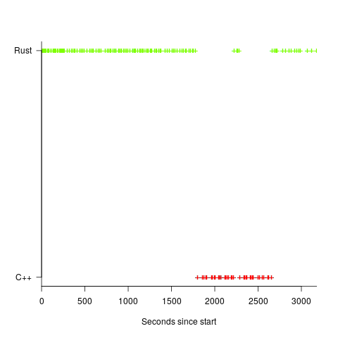
It is possible that one or more background processes were running while one set of language benchmarks was being run, which would skew the results. One solution is to intermix the runs for each language (switching off all background tasks is much harder).
I was surprised by how well the regression model fitted the data; the fit is rarely this good. Perhaps a larger set of benchmarks would increase the variance.
Recent Comments