Archive
Median system cpu clock frequency over last 15 years
We are all familiar with graphs showing the growth of cpu clock frequency over time. The data for these plots is based on vendor announcements listing the characteristics of their latest products, and invariably focuses on the product which is the fastest or contains the most transistors or the lowest power consumption.
Some customers buy the cpu with the highest/most/lowest, but many are happy to pay less for, for good enough. What does a graph of average customer cpu clock frequency over time look like?
Vendors sometimes publish general sales figures, but I have never seen one broken down by clock frequency. However, a few sites collect user system data, including:
- A subset of the Linux Counter project data is available. This does not contain explicit date information, but a must-be-later-than date can be inferred from the listed Linux kernel version,
- Hardware for BSD has data going back to December 2014, but there is no obvious way to extract it (I have not tried that hard),
- the BSDstats project (variable website availability) has been collecting data on machines running some derivative of BSD since August 2008; it contains around 200 times more cpu data than the known Linux Counter data. While the raw data is not available, approximately monthly reports are available on the Wayback Machine.
A BSDstats cpu history was obtained using waybackpack to download the available stored cpu summary pages, followed by html2text, and an awk script to extract the cpu frequency/count data.
BSDstats obtains the cpu information via a call to the sysctl command. For many Intel processors, but not AMD processors, the returned string includes the frequency (to see your cpu information on Linux systems type: more /proc/cpu), for instance:
Celeron(R) CPU 2.80GHz | 336 Pentium(R) 4 CPU 3.00GHz | 258 Pentium(R) 4 CPU 2.40GHz | 170 Athlon(tm) 64 Processor 3000+ | 43 Athlon(tm) 64 X2 Dual Core Processor 4200+ | 28 Athlon(tm) 64 Processor 3500+ | 27 |
For simplicity, only those rows containing frequency information were used in this analysis; 67% of the strings explicitly included a frequency (this saved me having to build a table to map AMD cpu strings to their corresponding frequency).
The plot below shows median cpu frequency (in red), along with the top/bottom 10% cpu frequencies, based on the Wayback Machine’s copy of the webpage on a given date, for a total of 2,304,446 cpu identities (code+data):
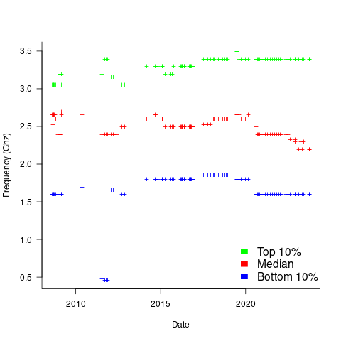
Broadly, the plot shows that cpu frequencies have essentially remained unchanged since 2008, with systems running BSD having a median frequency of 2.5 GHz, with 10% of systems having a frequency over 3.5 GHz, and 10% of systems a frequency below 1.5 GHz.
I was surprised at how many different frequencies were present in the data; often over 50. A look at the large number of different versions of Intel x86 cpus suggests that this is to be expected.
How representative is this sample of BSD systems, compared to the many more systems running Linux and Windows?
This begs the question of what kinds of environments are being compared. Are these desktop systems, local or hosted clusters, cloud systems?
The plot below shows the total number of cpus summarised on each Wayback Machine snapshot (code+data):
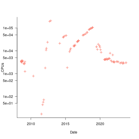
A few thousand systems are likely to be personal desktop systems, while the tens of thousands are likely to be clusters or small cloud providers.
Pointers to more data, particularly pre-2000, most welcome.
Testing rounded data for a circular uniform distribution
Circular statistics deals with analysis of measurements made using a circular scale, e.g., minutes past the hour, days of the week. Wikipedia uses the term directional statistics, the traditional use being measurements of angles, e.g., wind direction.
Package support for circular statistics is rather thin on the ground. R’s circular package is one of the best, and the book “Circular Statistics in R” provides the only best introduction to the subject.
Circular statistics has a few surprises for those new to the subject (apart from a few name changes, e.g., the von Mises distribution is effectively the ‘circular Normal distribution’), including:
- the mean value contains two components, a direction and a length, e.g., mean wind direction and strength,
- there are several definitions of variance, with angular variance having a value between 0 and 2, and circular variance having a value between 0 and 1. The circular standard deviation is not the square root of variance, but rather:
 , where
  is the mean length.
The basic techniques used in circular statistics are still relatively new, compared to the more well known basic statistical techniques. For instance, it was recently discovered that having more measurements may reduce the reliability of the Rao spacing test (used to test whether a sample has a uniform circular distribution); generally, having more measurements improves the reliability of a statistical test.
The plot below shows Rose diagrams for the number of commits in each 3-hour period of a day for Linux and FreeBSD (mean direction and length in green; code+data):
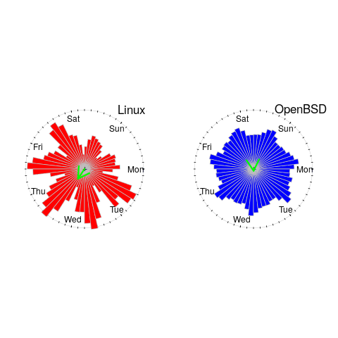
The Linux kernel source has far fewer commits at the weekend, compared to working days. Given the number of people whose job is to work on the Linux kernel, compared to the number of people doing it out of interest, this difference is not surprising. The percentage of people working on OpenBSD as a job is small, and there does not appear to be a big difference between weekends and workdays. There is a lot of variation in the number of commits during each 3-hour period of a day, but the number of commits per day does not vary so much; the number of OpenBSD commits per day of week is:
            Mon   Tue   Wed   Thu   Fri   Sat   Sun
26909 26144 25705 25104 24765 22812 24304 |
Does this distribution of commits per day have a uniform distribution (to some confidence level)?
Like all measurements, those made on a circular scale are rounded to some number of digits. Measurements may also be rounded, or binned, to particular units of the scale, e.g., measured to the nearest degree, or nearest minute.
A recent paper, by Landler, Ruxton and Malkemper, found that for samples containing around five hundred or more measurements, rounding to the nearest degree was sufficient to cause the Rao spacing test to almost always report non-uniformity, i.e., for non-trivial samples the rounding was sufficient to cause the test to detect non-uniformity (things worked as expected for samples containing fewer than 100 measurements).
Landler et al found that adding a small amount of noise (drawn from a von Mises distribution) to the rounded measurements appeared to ‘fix’ the incorrect behavior, i.e., rejecting the hypothesis of a uniform distribution, when a uniform distribution may be present.
The rao.spacing.test function, in the circular package, rejected that null hypothesis that the OpenBSD daily data has a uniform distribution. However, when noise is added to each day value (i.e., adding a random fraction to the day values, using rvonmises(length(c_per_day), circular(0), 2.0), although runif(length(c_per_day)) is probably more appropriate {and produces essentially the same result}), the call to rao.spacing.test failed to reject the null hypothesis of uniformity at the 0.05 level (i.e., the daily distribution is probably uniform).
How many research results are affected by this discovery?
I very rarely encounter the use of circular statistics (even though they should probably have been used in places), but then I spend my time reading software engineering papers, whose use of statistics tends to be primitive. I plan to include a brief mention of the use of the Rao spacing test with binned data in the addendum to my Evidence-based software engineering book (which includes the above example).
Popularity of Open source Operating systems over time
Surveys of operating system usage trends are regularly published and we get to read about how the various Microsoft products are doing and the onward progress of mobile OSs; sometimes Linux gets an entry at the bottom of the list, sometimes it is just ‘others’ and sometimes it is both.
Operating systems are pervasive and a variety of groups actively track reported faults in order to issue warnings to the public; the volume of OS fault informations available makes it an obvious candidate for testing fault prediction models (e.g., how many faults will occur in a given period of time). A very interesting fault history analysis of OpenBSD in a paper by Ozment and Schechter recently caught my eye and I wondered if the fault time-line could be explained by the time-line of OpenBSD usage (e.g., more users more faults reported). While collecting OS usage information is not the primary goal for me I thought people would be interested in what I have found out and in particular to share the OS usage data I have managed to obtain.
How might operating system usage be measured? Analyzing web server logs is an obvious candidate method; when a web browser requests information many web servers write information about the request to a log file and this information sometimes includes the name of the operating system on which the browser is running.
Other sources of information include items sold (licenses in Microsoft’s case, CDs/DVD’s for Open source or perhaps books {but book sales tend not to be reported in the way programming language book sales are reported}) and job adverts.
For my time-line analysis I needed OpenBSD usage information between 1998 and 2005.
The best source of information I found, by far, of Open source OS usage derived from server logs (around 138 million Open source specific entries) is that provided by Distrowatch who count over 700 different distributions as far back as 2002. What is more Ladislav Bodnar the founder and executive editor of DistroWatch was happy to run a script I sent him to extract the count data I was interested in (I am not duplicating Distrowatch’s popularity lists here, just providing the 14 day totals for OS count data). Some analysis of this data below.
As luck would have it I recently read a paper by Diomidis Spinellis which had used server log data to estimate the adoption of Open Source within organizations. Diomidis researches Open source and was willing to run a script I wrote to extract the User Agent string from the 278 million records he had (unfortunately I cannot make this public because it might contain personal information such as email addresses, just the monthly totals for OS count data, tar file of all the scripts I used to process this raw log data; the script to try on your own logs is countos.sh).
My attempt to extract OS names from the list of User Agent strings Diomidis sent me (67% of of the original log entries did contain a User Agent string) provides some insight into the reliability of this approach to counting usage (getos.awk is the script to try on the strings extracted with the earlier script). There is no generally agreed standard for:
- what information should be present; 6% of UA strings contained no OS name that I knew (this excludes those entries that were obviously robots/crawlers/spiders/etc),
- the character string used to specify a given OS or a distribution; the only option is to match a known list of names (OS names used by Distrowatch,
missos.awkis the tar file script to print out any string not containing a specified list of OS names, the Wikipedia List of operating systems article), - quality assurance; some people cannot spell ‘windows’ correctly and even though the source is now available I don’t think anybody uses CP/M to access the web (at least 91 strings,
 %, would not have passed).
Ladislav Bodnar thinks that log entries from the same IP addresses should only be counted once per day per OS name. I agree that this approach is much better than ignoring address information; why should a person who makes 10 accesses be counted 10 times, a person who makes one access is only counted once. It is possible that two or more separate machines running the same OS are accessing the Internet through a common gateway that results in them having the IP address from an external server’s point of view; this possibility means that the Distrowatch data undercounts the unique accesses (not a serious problem if most visitors have direct Internet access rather than through a corporate network).
The Distrowatch data includes counts for all IP address and from 13 May 2004 onwards unique IP address per day per OS. The mean ratio between these two values, summed over all OS counts within 14 day periods, is 1.9 (standard deviation 0.08) and the Pearson correlation coefficient between them is 0.987 (95% confidence interval is 0.984 to 0.990), i.e., almost perfect correlation.
The Spinellis data ignores IP address information (I got this dataset first, and have already spent too much time collecting to do more data extraction) and has 10 million UA strings containing Open source OS names (6% of all OS names matched).
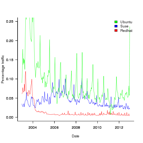
How representative are the Distrowatch and Spinellis data? The data is as representative of the general OS population as the visitors recorded in the respective server logs are representative of OS usage. The plot below shows the percentage of visitors to Distrowatch that use Ubuntu, Suse, Redhat. Why does Redhat, a very large company in the Open source world, have such a low percentage compared to Ubuntu? I imagine because Redhat customers get their updates from Redhat and don’t see a need to visit sites such as Distrowatch; a similar argument can be applied to Suse. Perhaps the Distrowatch data underestimates those distributions that have well known websites and users who have no interest in other distributions. I have not done much analysis of the Spinellis data.
Presumably the spikes in usage occur around releases of new versions, I have not checked.
For my analysis I am interested in relative change over time, which means that representativeness and not knowing the absolute number of OSs in use is not a problem. Researchers interested in a representative sample or estimating the total number of OSs in use are going to need a wider selection of data; they might be interested in the following OS usage information I managed to find (yes I know about Netcraft, they charge money for detailed data and I have not checked what the Wayback Machine has on file):
- Wikimedia has OS count information back to 2009. Going forward this is a source of log data to rival Distrowatch’s, but the author of the scripts probably ought to update the list of OS names matched against,
- w3schools has good summary data for many months going back to 2003,
- statcounter has good summary data (daily, weekly, monthly) going back to 2008,
- TheCounter.com had data from 2000 to 2009 (csv file containing counts obtained from Wayback Machine).
If any reader has or knows anybody who has detailed OS usage data please consider sharing it with everybody.
Recent Comments