Archive
Growth in FLOPs used to train ML models
AI (a.k.a. machine learning) is a compute intensive activity, with the performance of trained models being dependent on the quantity of compute used to train the model.
Given the ongoing history of continually increasing compute power, what is the maximum compute power that might be available to train ML models in the coming years?
How might the compute resources used to train an ML model be measured?
One obvious answer is to specify the computers used and the numbers of days used they were occupied training the model. The problem with this approach is that the differences between the computers used can be substantial. How is compute power measured in other domains?
Supercomputers are ranked using FLOPS (floating-point operations per second), or GigFLOPS or PetaFLOPS ( ). The Top500 list gives values for
  (based on benchmark performance, i.e., LINNPACK) and
  (what the hardware is theoretically capable of, which is sometimes more than twice ).
A ballpark approach to measuring the FLOPs consumed by an application is to estimate the FLOPS consumed by the computers involved and multiply by the number of seconds each computer was involved in training. The huge assumption made with this calculation is that the application actually consumes all the FLOPS that the hardware is capable of supplying. In some cases this appears to be the metric used to estimate the compute resources used to train an ML model. Some published papers just list a FLOPs value, while others list the number of GPUs used (e.g., 2,128).
A few papers attempt a more refined approach. For instance, the paper describing the GPT-3 models derives its FLOPs values from quantities such as the number of parameters in each model and number of training tokens used. Presumably, the research group built a calibration model that provided the information needed to estimate FLOPS in this way.
How does one get to be able to use PetaFLOPS of compute to train a model (training the GPT-3 175B model consumed 3,640 PetaFLOP days, or around a few days on a top 8 supercomputer)?
Pay what it costs. Money buys cloud compute or bespoke supercomputers (which are more cost-effective for large scale tasks, if you have around £100million to spend plus £10million or so for the annual electricity bill). While the amount paid to train a model might have lots of practical value (e.g., can I afford to train such a model), researchers might not be keen to let everybody know how much they spent. For instance, if a research team have a deal with a major cloud provider to soak up any unused capacity, those involved probably have no interest in calculating compute cost.
How has the compute power used to train ML models increased over time? A recent paper includes data on the training of 493 models, of which 129 include estimated FLOPs, and 106 contain date and model parameter data. The data comes from published papers, and there are many thousands of papers that train ML models. The authors used various notability criteria to select papers, and my take on the selection is that it represents the high-end of compute resources used over time (which is what I’m interested in). While they did a great job of extracting data, there is no real analysis (apart from fitting equations).
The plot below shows the FLOPs training budget used/claimed/estimated for ML models described in papers published on given dates; lines are fitted regression models, and the colors are explained below (code+data):
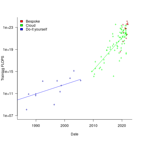
My interpretation of the data is based on the economics of accessing compute resources. I see three periods of development:
- do-it yourself (18 data points): During this period most model builders only had access to a university computer, desktop machines, or a compute cluster they had self-built,
- cloud (74 data points): Huge on demand compute resources are now just a credit card away. Researchers no longer have to wait for congested university computers to become available, or build their own systems.
AWS launched in 2006, and the above plot shows a distinct increase in compute resources around 2008.
- bespoke (14 data points): if the ML training budget is large enough, it becomes cost-effective to build a bespoke system, e.g., a supercomputer. As well as being more cost-effective, a bespoke system can also be specifically designed to handle the characteristics of the kinds of applications run.
How might models trained using a bespoke system be distinguished from those trained using cloud compute? The plot below shows the number of parameters in each trained model, over time, and there is a distinct gap between
 and
and  parameters, which I assume is the result of bespoke systems having the memory capacity to handle more parameters (code+data):
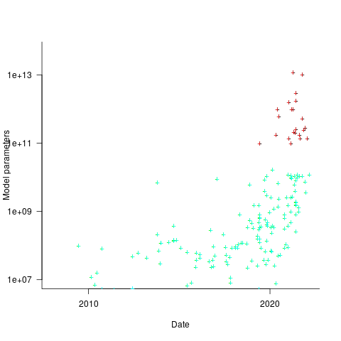
The rise in FLOPs growth rate during the Cloud period comes from several sources: 1) the exponential decline in the prices charged by providers delivers researchers an exponentially increasing compute for the same price, 2) researchers obtaining larger grants to work on what is considered to be an important topic, 3) researchers doing deals with providers to make use of excess capacity.
The rate of growth of Cloud usage is capped by the cost of building a bespoke system. The future growth of Cloud training FLOPs will be constrained by the rate at which the prices charged for a FLOP decreases (grants are unlikely to continually increase substantially).
The rate of growth of the Top500 list is probably a good indicator of the rate of growth of bespoke system performance (and this does appear to be slowing down). Perhaps specialist ML training chips will provide performance that exceeds that of the GPU chips currently being used.
The maximum compute that can be used by an application is set by the reliability of the hardware and the percentage of resources used to recover from hard errors that occur during a calculation. Supercomputer users have been facing the possibility of hitting the wall of maximum compute for over a decade. ML training is still a minnow in the supercomputer world, where calculations run for months, rather than a few days.
Software effort estimation is mostly fake research
Effort estimation is an important component of any project, software or otherwise. While effort estimation is something that everybody in industry is involved with on a regular basis, it is a niche topic in software engineering research. The problem is researcher attitude (e.g., they are unwilling to venture into the wilds of industry), which has stopped them acquiring the estimation data needed to build realistic models. A few intrepid people have risked an assault on their ego and talked to people in industry, the outcome has been, until very recently, a small collection of tiny estimation datasets.
In a research context, the term effort estimation is actually a hang over from the 1970s; effort correction more accurately describes the behavior of most models since the 1990s. In the 1970s, models took various quantities (e.g., estimated lines of code) and calculated an effort estimate. Later models have included an estimate as input to the model, producing a corrected estimate as output. For the sake of appearances, I will use existing terminology.
Which effort estimation datasets do researchers tend to use?
A 2012 review of datasets used for effort estimation using machine learning between 1991-2010, found that the top three were: Desharnias with 24 papers (29%), COCOMO with 19 papers (23%) and ISBSG with 17. A 2019 review of datasets used for effort estimation using machine learning between 1991 and 2017, found the top three to be NASA with 17 papers (23%), the COCOMO data and ISBSG were joint second with 16 papers (21%), and Desharnais was third with 14. The 2012 review included more sources in its search than the 2019 review, and subjectively your author has noticed a greater use of the NASA dataset over the last five years or so.
How large are these datasets that have attracted so many research papers?
The NASA dataset contains 93 rows (that is not a typo, there is no power-of-ten missing), COCOMO 63 rows, Desharnais 81 rows, and ISBSG is licensed by the International Software Benchmarking Standards Group (academics can apply for a limited time use for research purposes, i.e., not pay the $3,000 annual subscription). The China dataset contains 499 rows, and is sometimes used (there is no mention of a supercomputer being required for this amount of data ;-).
Why are researchers involved in software effort estimation feeding tiny datasets from the 1980s-1990s into machine learning algorithms?
Grant money. Research projects are more likely to be funded if they use a trendy technique, and for the last decade machine learning has been the trendiest technique in software engineering research. What data is available to learn from? Those estimation datasets that were flogged to death in the 1990s using non-machine learning techniques, e.g., regression.
Use of machine learning also has the advantage of not needing to know anything about the details of estimating software effort. Everything can be reduced to a discussion of the machine learning algorithms, with performance judged by a chosen error metric. Nobody actually looks at the predicted estimates to discover that the models are essentially producing the same answer, e.g., one learner predicts 43 months, 2 weeks, 4 days, 6 hours, 47 minutes and 11 seconds, while a ‘better’ fitting one predicts 43 months, 2 weeks, 2 days, 6 hours, 27 minutes and 51 seconds.
How many ways are there to do machine learning on datasets containing less than 100 rows?
A paper from 2012 evaluated the possibilities using 9-learners times 10 data-preprocessing options (e.g., log transform or discretization) times 7-error estimation metrics giving 630 possible final models; they picked the top 10 performers.
This 2012 study has not stopped researchers continuing to twiddle away on the option’s nobs available to them; anything to keep the paper mills running.
To quote the authors of one review paper: “Unfortunately, we found that very few papers (including most of our own) paid any attention at all to properties of the data set.”
Agile techniques are widely used these days, and datasets from the 1990s are not applicable. What datasets do researchers use to build Agile effort estimation models?
A 2020 review of Agile development effort estimation found 73 papers. The most popular data set, containing 21 rows, was used by nine papers. Three papers used simulated data! At least some authors were going out and finding data, even if it contains fewer rows than the NASA dataset.
As researchers in business schools have shown, large datasets can be obtained from industry; ISBSG actively solicits data from industry and now has data on 9,500+ projects (as far as I can tell a small amount for each project, but that is still a lot of projects).
Are there any estimates on GitHub? Some Open source projects use JIRA, which includes support for making estimates. Some story point estimates can be found on GitHub, but the actuals are missing.
A handful of researchers have obtained and released estimation datasets containing thousands of rows, e.g., the SiP dataset contains 10,100 rows and the CESAW dataset contains over 40,000 rows. These datasets are generally ignored, perhaps because when presented with lots of real data, researchers have no idea what to do with it.
Learning useful stuff from the Reliability chapter of my book
What useful, practical things might professional software developers learn from my evidence-based software engineering book?
Once the book is officially released I need to have good answers to this question (saying: “Well, I decided to collect all the publicly available software engineering data and say something about it”, is not going to motivate people to read the book).
This week I checked the reliability chapter; what useful things did I learn (combined with everything I learned during all the other weeks spent working on this chapter)?
A casual reader skimming the chapter would conclude that little was known about software reliability, and they would be right (I already knew this, but I learned that we know even less than I thought was known), and many researchers continue to dig in unproductive holes.
A reader with some familiarity with reliability research would be surprised to see that some ‘major’ topics are not discussed.
The train wreck that is machine learning has been avoided (not forgetting that the data used is mostly worthless), mutation testing gets mentioned because of some interesting data (the underlying problem is that mutation testing assumes that coding mistakes are local to one line, but in practice coding mistakes often involve multiple lines), and the theory discussions don’t mention non-homogeneous Poisson process as the basis for software fault models (because this process is not capable of solving the questions asked).
What did I learn? My highlights include:
- Anne Choa‘s work on population estimation. The takeaway from this work is that if people want to estimate the number of remaining fault experiences, based on previous experienced faults, then every occurrence (i.e., not just the first) of a fault needs to be counted,
- Phyllis Nagel and Janet Dunham’s top read work on software testing,
- the variability in the numeric percentage that people assign to probability terms (e.g., almost all, likely, unlikely) is much wider than I would have thought,
- the impact of the distribution of input values on fault experiences may be detectable,
- really a lowlight, but there is a lot less publicly available data than I had expected (for the other chapters there was more data than I had expected).
The last decade has seen fuzzing grow to dominate the headlines around software reliability and testing, and provide data for people who write evidence-based books. I don’t have much of a feel for how widely used it is in industry, but it is a very useful tool for reliability researchers.
Readers might have a completely different learning experience from reading the reliability chapter. What useful things did you learn from the reliability chapter?
The Algorithmic Accountability Act of 2019
The Algorithmic Accountability Act of 2019 has been introduced to the US congress for consideration.
The Act applies to “person, partnership, or corporation” with “greater than $50,000,000 … annual gross receipts”, or “possesses or controls personal information on more than— 1,000,000 consumers; or 1,000,000 consumer devices;”.
What does this Act have to say?
(1) AUTOMATED DECISION SYSTEM.—The term ‘‘automated decision system’’ means a computational process, including one derived from machine learning, statistics, or other data processing or artificial intelligence techniques, that makes a decision or facilitates human decision making, that impacts consumers.
That is all encompassing.
The following is what the Act is really all about, i.e., impact assessment.
(2) AUTOMATED DECISION SYSTEM IMPACT ASSESSMENT.—The term ‘‘automated decision system impact assessment’’ means a study evaluating an automated decision system and the automated decision system’s development process, including the design and training data of the automated decision system, for impacts on accuracy, fairness, bias, discrimination, privacy, and security that includes, at a minimum—
I think there is a typo in the following: “training, data” -> “training data”
(A) a detailed description of the automated decision system, its design, its training, data, and its purpose;
How many words are there in a “detailed description of the automated decision system”, and I’m guessing the wording has to be something a consumer might be expected to understand. It would take a book to describe most systems, but I suspect that a page or two is what the Act’s proposers have in mind.
(B) an assessment of the relative benefits and costs of the automated decision system in light of its purpose, taking into account relevant factors, including—
Whose “benefits and costs”? Is the Act requiring that companies do a cost benefit analysis of their own projects? What are the benefits to the customer, compared to a company not using such a computerized approach? The main one I can think of is that the customer gets offered a service that would probably be too expensive to offer if the analysis was done manually.
The potential costs to the customer are listed next:
(i) data minimization practices;
(ii) the duration for which personal information and the results of the automated decision system are stored;
(iii) what information about the automated decision system is available to consumers;
This act seems to be more about issues around data retention, privacy, and customers having the right to find out what data companies have about them
(iv) the extent to which consumers have access to the results of the automated decision system and may correct or object to its results; and
(v) the recipients of the results of the automated decision system;
What might the results be? Yes/No, on a load/job application decision, product recommendations are a few.
Some more potential costs to the customer:
(C) an assessment of the risks posed by the automated decision system to the privacy or security of personal information of consumers and the risks that the automated decision system may result in or contribute to inaccurate, unfair, biased, or discriminatory decisions impacting consumers; and
What is an “unfair” or “biased” decision? Machine learning finds patterns in data; when is a pattern in data considered to be unfair or biased?
In the UK, the sex discrimination act has resulted in car insurance companies not being able to offer women cheaper insurance than men (because women have less costly accidents). So the application form does not contain a gender question. But the applicants first name often provides a big clue, as to their gender. So a similar Act in the UK would require that computer-based insurance quote generation systems did not make use of information on the applicant’s first name. There is other, less reliable, information that could be used to estimate gender, e.g., height, plays sport, etc.
Lots of very hard questions to be answered here.
Facebook’s Big Code Summit
I was at Facebook’s first Big Code Summit on Monday and Tuesday (I say the first, because I hope there is another one next year).
The talks all involved machine learning (to be expected, given the Big Code in the event’s title). Normally I ignore papers on machine learning in software engineering, but understanding code is hard and we don’t know much about it. As I keep telling anyone who will listen, machine learning is the tool to use when you don’t know what you are doing (provided you have enough data).
People have been learning code patterns for some time now, suggesting applications in code completion in the IDE and finding suspicious API sequences (e.g., a missing call). This is one area where machine learning is a natural solution: nobody has the time to write down all the common patterns, for all the common languages, and APIs are constantly changing. It makes no sense to solve this problem manually.
So what was new and/or interesting?
We got new and very interesting in the first talk, when Eran Yahav presented his group’s work on cod2vec, the paper was interesting, but the demo had the wow factor.
I have not made up my mind about Michael Pradel‘s proposal for learning new coding rule checks. These rules are often created by people, but people with the necessary skill are thin on the ground. Machine learning requires something to learn from, how could coding rules be created this way. Michael’s group is working on a system where developers create the positive and negative cases and a machine learner figures out rules from these examples. Would the creation of these positive/negative examples prove to be just as hard as writing rules? I was not convinced that such an approach was practical, but if somebody wants to try it out, why not.
I found Xinyun Chen‘s talk interesting, but then I’ve written lots of parsers, and automatically figuring out how to parse a language from examples will always get my attention. A few people in the audience thought that a better solution was typing in a grammar and parsing the ‘usual’ way. This approach assumes a grammar exists, can be strong-armed into a form that is practical to embed in a parser (requiring somebody skilled in the necessary black arts), to produce a system that will only process complete translation units (or whatever the language calls a unit of translation).
Finding the gold nugget papers in software engineering research
Academic research projects are like startups in that most fail to make any return on their investment (e.g., the tax payer does not get any money back) and a few pay for themselves and all the failures. Irrespective of whether a project succeeds or fails, those involved will publish papers on the work, give talks at conferences and workshops and general try to convince anyone who will listen that the project was a great success.
Number or papers published plays an important role in evaluating the quality of a university department and the performance on an individual researcher. As you can imagine, this publish or perish culture leads to huge amounts of clueless nonsense ending up in print. Don’t be fooled by the ‘peer reviewed’ label, most of this gets done by the least experienced people (e.g., postgrad students) as a means of gaining social recognition in their specific research community, i.e., those doing the reviewing don’t always know much.
The huge number of papers describing failed projects and/or containing clueless nonsense is a major obstacle for anyone wanting to locate useful new knowledge.
While writing my C book I refined the following approach to finding high quality papers and created filtering rules for the subjects it covered. The rules below are being applied to papers relating to my Empirical Software Engineering book. I don’t claim any usefulness for these rules outside of academic software engineering research.
I use a scatter gun approach to obtain a basic collection of papers followed by ruthless filtering.
The scatter gun approach might start with one or two papers; following links on Google Scholar or even just Google search results filtered on “filetype:pdf”, in the past I have used CiteSeer which Google now does a better job of indexing, and Semantic Scholar is now starting to be quite good.
After 30 minutes or so I have 50 pdfs (I download maybe 4,000 a year). Now I need to quickly filter the nonsense to end up with maybe 10 that I will spend 5 minutes each reading, leaving maybe 2 or 3 for detailed reading (often not the original ones I started with).
When dealing with this kind of volume you have to be ruthless.
Spend just 10 seconds on the first pass. If a paper has some merits, let it remain for the next pass. Scan the paper looking for major indicators of clueless nonsense; these are not hard to spot, don’t linger, hit the delete (if data is involved, it is worth quickly checking the footnotes for a url to a dataset, which may be new and worth collecting):
- it relies on machine learning,
- it relies on information theory,
- it relies on Halstead’s metric,
- it investigates software quality. This is a marketing term used to give a patina of relevance to the worthless metric that is likely used in the research. Be on the lookout for other high relevance terms being used to provide a positive association with a worthless metric, e.g., developer productivity defined as volume of code written
- it involves fault prediction. Academic folk psychology includes a belief that some project files contain more faults than other files, because more faults are reported in some files than others (or even that entire projects are more reliable because fewer faults have been reported). This is a case of the drunk searching under a streetlight for lost keys because that is where the ground can be seen. Faults are found by executing code, more execution means more faults. I only know of two papers that are exceptions to this rule (one of them is discussed here),
- the primary claim in the conclusion is to have done something novel. Research requires doing new stuff, novel is a key attribute that is rather pointless for its own sake. Typing code using your nose would be novel, but would you want to spend more than 10 seconds reading a paper on the subject (and this example is at the more sensible end of the spectrum of novel research I have read about).
The first pass removes around 70-80% of the papers, at least for me.
For the second pass I will spend a minute or so doing a slightly slower scan. This often cuts the papers remaining in half.
By now, I have been collecting and filtering for over 90 minutes; time to do something else, perhaps not returning for many hours.
The third pass involves trying to read the paper. The question is: Am I having trouble reading this paper because the author has managed to compress a lot of useful information into a publication page limit, or is the paper so bad I cannot see the wood for the dead trees?
Answering this question takes practice and some knowledge of the subject area. You will speed up with practice and learning about the subject.
Some things that might be thought worth paying attention to, but should be ignored:
- don’t bother looking at the names of the authors or which university they work at (who wrote the paper almost always provides no clues to its quality; there are very few exceptions to this and you will learn who they are over time),
- ignore the journal or conference that published the paper (gold nuggets appear everywhere and high impact venues only restrict the clueless nonsense to the current trendy topics and papers citing the ‘right’ people),
- ignore year of publication, quality is ageless (and sometimes fades from view because research fashions change).
If you have your own tips for finding the gold nuggets in software engineering, please let me know.
Machine learning in SE research is a bigger train wreck than I imagined
I am at the CREST Workshop on Predictive Modelling for Software Engineering this week.
Magne Jørgensen, who virtually single handed continues to move software cost estimation research forward, kicked-off proceedings. Unfortunately he is not a natural speaker and I think most people did not follow the points he was trying to get over; don’t panic, read his papers.
In the afternoon I learned that use of machine learning in software engineering research is a bigger train wreck that I had realised.
Machine learning is great for situations where you have data from an application domain that you don’t know anything about. Lets say you want to do fault prediction but don’t have any practical experience of software engineering (because you are an academic who does not write much code), what do you do? Well you could take some source code measurements (usually on a per-file basis, which is a joke given that many of the metrics often used only have meaning on a per-function basis, e.g., Halstead and cyclomatic complexity) and information on the number of faults reported in each of these files and throw it all into a machine learner to figure the patterns and build a predictor (e.g., to predict which files are most likely to contain faults).
There are various ways of measuring the accuracy of the predictions made by a model and there is a growing industry of researchers devoted to publishing papers showing that their model does a better job at prediction than anything else that has been published (yes, they really do argue over a percent or two; use of confidence bounds is too technical for them and would kill their goose).
I long ago learned to ignore papers on machine learning in software engineering. Yes, sooner or later somebody will do something interesting and I will miss it, but will have retained my sanity.
Today I learned that many researchers have been using machine learning “out of the box”, that is using whatever default settings the code uses by default. How did I learn this? Well, one of the speakers talked about using R’s carat package to tune the options available in many machine learners to build models with improved predictive performance. Some slides showed that the performance of carat tuned models were often substantially better than the non-carat tuned model and many people in the room were aghast; “If true, this means that all existing papers [based on machine learning] are dead” (because somebody will now come along and build a better model using carat; cannot recall whether “dead” or some other term was used, but you get the idea), “I use the defaults because of concerns about breaking the code by using inappropriate options” (obviously somebody untroubled by knowledge of how machine learning works).
I think that use of machine learning, for the purpose of prediction (using it to build models to improve understanding is ok), in software engineering research should be banned. Of course there are too many clueless researchers who need the crutch of machine learning to generate results that can be included in papers that stand some chance of being published.
Never too experienced to make a basic mistake
I was one of the 170 or so people at the Data Science hackathon in London over the weekend. As always this was well run by Carlos and his team who kept us fed, watered and connected to the Internet.
One of the three challenges involved a dataset containing pairs of Twitter users, A and B, where one of the pair had been ranked, by a person, as more influential than the other (the data was provided by PeerIndex, an event sponsor). The dataset contained 22 attributes, 11 for each user of the pair, plus 0/1 to indicate who was most influential; there was a training dataset of 5.5K pairs to learn against and a test dataset to make predictions against. The data was not messy or even sparse, how hard could it be?
Talks had been organized for the morning and afternoon. While Microsoft (one of the event sponsors) told us about Azure and F#, I sat at the back trying out various machine learning packages. Yes, the technical evangelists told us, Linux as well as Windows instances were available in Azure, support was available for the usual big data languages (e.g., Python and R; the Microsoft people seemed to be much more familiar with Python) plus dot net (this was the first time I had heard the use of dot net proposed as a big data solution for the Cloud).
Some members of Team Outliers from previous hackathons (Jonny, Bob and me) formed a team and after the talks had finished the Microsoft people+partners sat at our table (probably because our age distribution was similar to theirs, i.e., at the opposite end of the range to most teams; some of the Microsoft people got very involved in trying to produce a solution to the visualization challenge).
Integrating F# with bigdata seems to involve providing an interface to R packages (this is done by interfacing to the packages installed on a local R installation) and getting the IDE to know about the names of columns contained in data that has been read. Since I think the world needs new general purpose programming languages as much as it needs holes in the head I won’t say any more.
When in challenge solving mode I was using cross-validation to check the models being built and scoring around 0.76 (AUC, the metric used by the organizers). Looking at the leader board later in the afternoon showed several teams scoring over 0.85, a big difference; what technique were they using to get such a big improvement?
A note: even when trained on data that uses 0/1 predictor values machine learners don’t produce models that return zero or one, many return values in the range 0..1 (some use other ranges) and the usual technique is treat all values greater than 0.5 as a 1 (or TRUE or ‘yes’, etc) and all other values as a 0 (or FALSE or ‘no’, etc). This (x > 0.5) test had to be done to cross validate models using the training data and I was using the same technique for the test data. With an hour to go in the 24 hour hackathon we found out (change from ‘I’ to ‘we’ to spread the mistake around) that the required test data output was a probability in the range 0..1, not just a 0/1 value; the example answer had this behavior and this requirement was explained in the bottom right of the submission page! How many times have I told others to carefully read the problem requirements? Thankfully everybody was tired and Jonny&Bob did not have the energy to throw me out of the window for leading them so badly astray.
Having AUC as the metric should have raised a red flag, this does not make much sense for a 0/1 answer; using AUC makes sense for PeerIndex because they will want to trade off recall/precision. Also, its a good idea to remove ones ego when asked the question: are lots of people doing something clever or are you doing something stupid?
While we are on the subject of doing the wrong thing, one of the top three teams gave an excellent example of why sales/marketing don’t like technical people talking to clients. Having just won a prize donated by Microsoft for an app using Azure, the team proceeded to give a demo and explain how they had done everything using Google services and made it appear within a browser frame as if it were hosted on Azure. A couple of us sitting at the back were debating whether Microsoft would jump in and disqualify them.
What did I learn that I did not already know this weekend? There are some R machine learning packages on CRAN that don’t include a predict function (there should be a research-only subsection on CRAN for packages like this) and some ranking algorithms need more than 6G of memory to process 5.5K pairs.
There seemed to be a lot more people using Python, compared to R. Perhaps having the sample solution in Python pushed the fence sitters that way. There also seemed to be more women present, but that may have been because there were more people at this event than previous ones and I am responding to absolute numbers rather than percentage.
Success does not require understanding
I took part in the second Data Science London Hackathon last weekend (also my second hackathon) and it was a very different experience compared to the first hackathon. Once again Carlos and his team really looked after us.
- The data was released 24 hours before the competition started and even though I had spent less than half an hour looking at it, at the start of the competition I did not feel under any time pressure; those 24 hours allowed me to get used to the data and come up with some useful looking ideas.
- The instructions for the first competition had suggested that people form teams of 3-5 and there was a lot of networking happening before the start time. There was no such suggestion this time and as I networked around looking for people to work with I was surprised by the number of people who wanted to work alone; Jonny and Kannappan were the only members from my previous team (the Outliers) who had entered this event, with Kannappan wanting to work alone and Jonny joining me to create a two person team.
- There was less community spirit this time, possible reasons include a lot more single person teams sitting in the corner doing their own thing, fewer people attending (it is the middle of the holiday season), fewer people staying over until the Sunday (perhaps single person teams got disheartened and left or the extra 24 hours of data access meant that teams ran out of ideas/commitment after 36 hours) or me being reduced to a single person team (Jonny had to leave at 20:00) meant I paid more attention to what was happening on the floor.
The problem was to predict what ratings different people would give to various music artists. We were given data involving 50 artists and 48,645 users (artists and users were anonymous) in five files (one contained the training dataset and another the test dataset).
A quick analysis of the data showed that while there were several thousand rows of data per artist there were only half a dozen rows per person, a very sparse dataset.
The most frequent technique I heard mentioned during my initial conversations with attendees was machine learning. In my line of work I am constantly trying to understand what is going on (the purpose of this understanding is to control and make things better) and consider anybody who uses machine learning as being clueless, dim witted or just plain lazy; the problem with machine learning is that it gives answers without explanations (ok decision trees do provide some insights). This insistence on understanding turned out to be my major mistake, the competition metric is based on correctness of answers and not on how well a competitor understands the problem domain. I had a brief conversation with a senior executive from EMI (who supplied the dataset and provided some of the sponsorship money) who showed up on Sunday morning and he had no problem with machine learning providing answers and not explanations.
Having been overly ambitious last time team Outliers went for extreme simplicity and started out with the linear model glm(Rating ~ AGE + GENDER...) being built for each artist (i.e., 50 models). For a small amount of work we got a score of just over 21 and a place of around 70th on the leader board, now we just needed to include information along the lines of “people who like Artist X also like Artist Y”. Unfortunately the only other member of my team (who did not share my view of machine learning and knew something about it) had a prior appointment and had to leave me consuming lots of cpu time on a wild goose chase that required me to have understanding.
The advantages of being in a team include getting feedback from other members (e.g., why are you wasting your time doing that, look how much better this approach is) and having access to different skill sets (e.g., knowing what magic pixie dust values to use for the optional parameters to machine learning routines). It was Sunday morning before I abandoned the ‘understanding’ approach and started thrashing around using various machine learning techniques, which told me that people demographics (e.g., age and gender) were not particularly good predictors compared to other data but did did not reduce my score to the 13-14 range that could be seen on the leader board’s top 20.
Realizing that seven hours was not enough time to learn how to drive R’s machine learning packages well enough to get me into the top ten, I switched tack and spent a lot more time wandering around chatting to people; those whose score was worse than mine were generally willing to chat. Some had gotten completely bogged down in data cleaning and figuring out how to handle missing data (a subject rarely covered in books but of huge importance in real life), I was surprised to find one team doing most of their coding in SQL (my suggestion to only consider Age+Gender improved their score from 35 to 22), I mocked the people using Clojure (people using a Lisp derived language think they have discovered the one true way and will suffer from self doubt if they are not mocked regularly). Afterwards it struck me that well over 50% of attendees were not British (based on their accents), was this yet another indicator of how far British Universities had dumbed down mathematics teaching that natives did not feel up to the challenge (well done to the Bristol undergraduate who turned up) or were the most gung-ho technical folk in London those who had traveled here to work from abroad?
The London winner was Dell Zhang, the only other person sitting at the table I was on (he sat opposite me throughout the competition), who worked quietly away for the whole 24 hours and seemed permanently unimpressed by the score he was achieving; he described his technique as “brute force random forest using Python (the source will be made available on the Data Science website).
Reading through posts made by competitors after the event was as interesting as last time. Factorization Machines seems to be the hot new technique for making predictions based on very sparse data and the libFM is the software I needed to know about last weekend (no R package providing an interface to this C++ code available yet).
Code generation via machine learning
Commercial compiler implementors have to produce compilers that are capable of being used on a typical developer computer. A whole bunch of optimization techniques were known for years but could not be used because few computers had the available memory capacity (in the days when 2M was a lot of memory your author once attended a talk that presented some impressive results and was frustrated to learn that the typical memory footprint was 160M, who would ever imagine developers having so much memory to work within?) These days the available of gigabytes of storage has means that likely computer storage capacity is rarely a reason not to use some optimization technique, although the whole program optimization people are still out in the cold.
What is new these days is the general availability of multiple processors. The obvious use of multiple processors is to have make distribute the compilation load. The more interesting use is having the compiler apply different sets of optimizations techniques on different processors, picking the one that produces the highest quality code.
Optimizing code generation algorithms don’t appear to leave anything to chance and individually they generally don’t. However, selecting an order in which to apply individual optimization algorithms is something of a black art. In some cases code transformations made by one algorithm can interfere with the performance of another algorithm. In some cases the possibility of the interference is known and applies in one direction, choosing the appropriate relative ordering of the two algorithms solves the problem. In other cases the way in which two algorithms interfere with each other depends on the code being translated, now the ordering of the two algorithms becomes problematic. The obvious solution is to try both orderings and pick the one that produces the best result.
Several research groups have investigated the use of machine learning in compiler optimization. cTuning.org is a new project that aims to bring together groups interested in self-tuning adaptive computing systems based on statistical and machine learning techniques.
Commercial pressure is always forcing compiler implementors to produce faster code and use of machine learning techniques can produce some impressive results. Now that multi-processor systems are common it will not be long before compilers writers start to make use of the extra resources now available to them.
The safety critical people have problems trying to show the correctness of compiler output that has been generated by ‘fixed’ algorithms. It is not hard to envisage that in 10 years time all large production quality compilers will be using machine learning.
Recent Comments