Archive
Average lines added/deleted by commits across languages
Are programs written in some programming language shorter/longer, on average, than when written in other languages?
There is a lot of variation in the length of the same program written in the same language, across different developers. Comparing program length across different languages requires a large sample of programs, each implemented in different languages, and by many different developers. This sounds like a fantasy sample, given the rarity of finding the same specification implemented multiple times in the same language.
There is a possible alternative approach to answering this question: Compare the size of commits, in lines of code, for many different programs across a variety of languages. The paper: A Study of Bug Resolution Characteristics in Popular Programming Languages by Zhang, Li, Hao, Wang, Tang, Zhang, and Harman studied 3,232,937 commits across 585 projects and 10 programming languages (between 56 and 60 projects per language, with between 58,533 and 474,497 commits per language).
The data on each commit includes: lines added, lines deleted, files changed, language, project, type of commit, lines of code in project (at some point in time). The paper investigate bug resolution characteristics, but does not include any data on number of people available to fix reported issues; I focused on all lines added/deleted.
Different projects (programs) will have different characteristics. For instance, a smaller program provides more scope for adding lots of new functionality, and a larger program contains more code that can be deleted. Some projects/developers commit every change (i.e., many small commit), while others only commit when the change is completed (i.e., larger commits). There may also be algorithmic characteristics that affect the quantity of code written, e.g., availability of libraries or need for detailed bit twiddling.
It is not possible to include project-id directly in the model, because each project is written in a different language, i.e., language can be predicted from project-id. However, program size can be included as a continuous variable (only one LOC value is available, which is not ideal).
The following R code fits a basic model (the number of lines added/deleted is count data and usually small, so a Poisson distribution is assumed; given the wide range of commit sizes, quantile regression may be a better approach):
alang_mod=glm(additions ~ language+log(LOC), data=lc, family="poisson") dlang_mod=glm(deletions ~ language+log(LOC), data=lc, family="poisson") |
Some of the commits involve tens of thousands of lines (see plot below). This sounds rather extreme. So two sets of models are fitted, one with the original data and the other only including commits with additions/deletions containing less than 10,000 lines.
These models fit the mean number of lines added/deleted over all projects written in a particular language, and the models are multiplicative. As expected, the variance explained by these two factors is small, at around 5%. The two models fitted are (code+data):
 or
or  , and
, and  or
or  , where the value of
  is listed in the following table, and
  is the number of lines of code in the project:
                    Original          0 < lines < 10000
    Language     Added     Deleted     Added   Deleted
    C              1.0       1.0         1.0     1.0
    C#             1.7       1.6         1.5     1.5
    C++            1.9       2.1         1.3     1.4
    Go             1.4       1.2         1.3     1.2
    Java           0.9       1.0         1.5     1.5
    Javascript     1.1       1.1         1.3     1.6
    Objective-C    1.2       1.4         2.0     2.4
    PHP            2.5       2.6         1.7     1.9
    Python         0.7       0.7         0.8     0.8
Ruby 0.3 0.3 0.7 0.7 |
These fitted models suggest that commit addition/deletion both increase as project size increases, by around  , and that, for instance, a commit in Go adds 1.4 times as many lines as C, and delete 1.2 as many lines (averaged over all commits). Comparing adds/deletes for the same language: on average, a Go commit adds
  lines, and deletes
  lines.
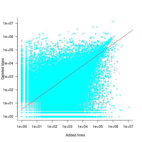
There is a strong connection between the number of lines added/deleted in each commit. The plot below shows the lines added/deleted by each commit, with the red line showing a fitted regression model  (code+data):
What other information can be included in a model? It is possible that project specific behavior(s) create a correlation between the size of commits; the algorithm used to fit this model assumes zero correlation. The glmer function, in the R package lme4, can take account of correlation between commits. The model component (language | project) in the following code adds project as a random effect on the language variable:
del_lmod=glmer(deletions ~ language+log(LOC)+(language | project), data=lc_loc, family=poisson) |
It takes around 24hr of cpu time to fit this model, which means I have not done much experimentation…
Some data on the size of Cobol programs/paragraphs
Before the internet took off in the 1990s, COBOL was the most popular language, measured in lines of code in production use. People who program in Cobol often have a strong business focus, and don’t hang out on sites used aggregated by surveys of programming language use; use of the language is almost completely invisible to those outside the traditional data processing community. So who knows how popular Cobol is today.
Despite the enormous quantity of Cobol code that has been written, very little Cobol source is publicly available (Open source or otherwise; the NIST compiler validation suite is not representative). The reason for the sparsity of source code is that Cobol programs are used to process business data, and the code is useless without the appropriate data (even with the data, the output is only likely to be of interest to a handful of people).
Program and function/method size (in LOC) are basic units of source code measurement. Until open source happened, published papers containing these measurements were based on small sample sizes and the languages covered was somewhat spotty. Cobol oriented research usually has a business orientation, rather than being programming oriented, and now there is a plentiful supply of source code written in non-Cobol languages.
I recently discovered appendix B of 1st Lt Richard E. Boone’s Master’s thesis An investigation into the use of software product metrics for COBOL systems (it’s post Rome period). Several days/awk scripts and editor macros later, LOC data for 178 programs containing 2,682 paragraphs containing 53,255 statements is now online (code+data).
A note on terminology: Cobol functions/methods are called paragraphs.
A paragraph is created by attaching a label to the first statement of the paragraph (there are no variables local to a paragraph; all variables are global). The statement PERFORM NAME-OF-PARAGRAPH ‘calls’ the paragraph labelled by NAME-OF-PARAGRAPH, somewhat like gosub number in BASIC.
It is possible to specify a sequence of paragraphs to be executed, in a PERFORM statement. The statement PERFORM NAME-OF-P1 THRU NAME-OF-P99 causes all paragraphs appearing textually in the code between the start of paragraph NAME-1 and the end of paragraph NAME-99 to be executed.
As far as I can tell, Boone’s measurements are based on individual paragraphs, not any sequences of paragraphs that are PERFORMed (it is likely that some labelled paragraphs are never PERFORMed in isolation).
Appendix B lists for each program: the paragraphs it contains, and for each paragraph the number of statements, McCabe’s complexity, maximum nesting, and Henry and Kafura’s Information flow metric
There are, based on naming, many EXIT paragraphs (711 or 26%); these are single statement paragraphs containing the statement EXIT. When encountered as the last paragraph of a PERFORM THU statement, the EXIT effectively acts like a procedure return statement; in other contexts, the EXIT statement acts like a continue statement.
In the following code the developer could have written PERFORM PARA-1 THRU PARA-4, but if a related paragraph was added between PARA-4 and PARA-END_EXIT all PERFORMs explicitly referencing PARA-4 would need to be checked to see if they needed updating to the new last paragraph.
START. PERFORM PARA-1 THRU PARA-END-EXIT. PARA-1. DISPLAY 'PARA-1'. PARA-2. DISPLAY 'PARA-2'. PARA-3. DISPLAY 'PARA-3'. P3-EXIT. EXIT. PARA-4. DISPLAY 'PARA-4'. PARA-END-EXIT. EXIT. |
The plot below shows the number of paragraphs containing a given number of statements, the red dot shows the count with EXIT paragraphs are ignored (code+data):

How does this distribution compare with that seen in C and Java? The plot below shows the Cobol data (in black, with frequency scaled-up by 1,000) superimposed on the same counts for C and Java (C/Java code+data):
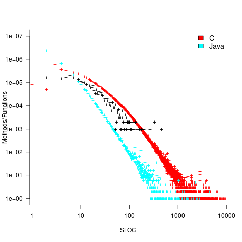
The distribution of statements per paragraph/function distribution for Cobol/C appears to be very similar, at least over the range 10-100. For less than 10-LOC the two languages have very different distributions. Is this behavior particular to the small number of Cobol programs measured? As always, more data is needed.
How many paragraphs does a Cobol program contain? The plot below shows programs ranked by the number of paragraphs they contain, including and excluding EXIT statements (code+data):
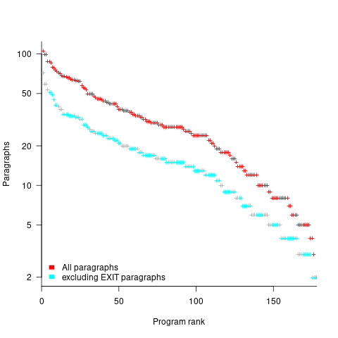
If you squint, it’s possible to imagine two distinct exponential declines, with the switch happening around the 100th program.
It’s tempting to draw some conclusions, but the sample size is too small.
Pointers to large quantities of Cobol source welcome.
Optimal function length: an analysis of the cited data
Careful analysis is required to extract reliable conclusions from data. Sloppy analysis can lead to incorrect conclusions being drawn.
The U-shaped plots cited as evidence for an ‘optimal’ number of LOC in a function/method that minimises the number of reported faults in a function, were shown to be caused by a mathematical artifact. What patterns of behavior are present in the data cited as evidence for an optimal number of LOC?
The 2000 paper Module Size Distribution and Defect Density by Malaiya and Denton summarises the data-oriented papers cited as sources on the issue of optimal length of a function/method, in LOC.
Note that the named unit of measurement in these papers is a module. In one paper, a module is specified as being as Ada package, but these papers specify that a module is a single function, method or anything else.
In order of publication year, the papers are:
The 1984 paper Software errors and complexity: an empirical investigation by Basili, and Perricone analyses measurements from a 90K Fortran program. The relevant Faults/LOC data is contained in two tables (VII and IX). Modules are sorted in to one of five bins, based on LOC, and average number of errors per thousand line of code calculated (over all modules, and just those containing at least one error); see table below:
     Module         Errors/1k lines   Errors/1k lines
     max LOC          all modules      error modules
        50              16.0               65.0
       100              12.6               33.3
       150              12.4               24.6
       200               7.6               13.4
>200 6.4 9.7 |
One of the paper’s conclusions: “One surprising result was that module size did not account for error proneness. In fact, it was quite the contrary–the larger the module, the less error prone it was.”
The 1985 paper Identifying error-prone software—an empirical study by Shen, Yu, Thebaut, and Paulsen analyses defect data from three products (written in Pascal, PL/S, and Assembly; there were three versions of the PL/S product) were analysed using Halstead/McCabe, plus defect density, in an attempt to identify error-prone software.
The paper includes a plot (figure 4) of defect density against LOC for one of the PL/S product releases, for 108 modules out of 253 (presumably 145 modules had no reported faults). The plot below shows defects against LOC, the original did not include axis values, and the red line is the fitted regression model  (data extracted using WebPlotDigitizer; code+data):
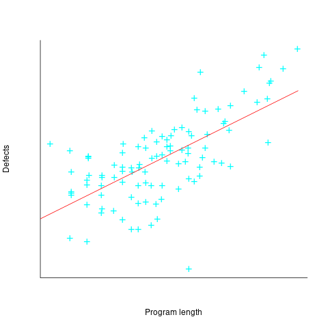
The power-law exponent is less than one, which suggests that defects per line is decreasing as module size increases, i.e., there is no optimal minimum, larger is always better. However, the analysis is incomplete because it does not include modules with zero reported defects.
The authors say: “… that there is a higher mean error rate in smaller sized modules, is consistent with that discovered by Basili and Perricone.”
The 1990 paper Error Density and Size in Ada Software by Carol Withrow analyses error data from a 114 KLOC military communication system written in Ada; of the 362 Ada packages, 137 had at least one error. The unit of measurement is an Ada package, which like a C++ class, can contain multiple definitions of types, variables, and functions.
The paper plots errors per thousand line of code against LOC, for packages containing at least one error, i.e., 62% of packages are not included in the analysis. The 137 packages are sorted into 8-bins, based on the number of lines they contain. The 52 packages in the 159-251 LOC bin have an average of 1.8 errors per 1 KLOC, which is the lowest bin average. The author concludes: “Our study of a large Ada project shows this optimal size to be about 225 lines.”
The plot below shows errors against LOC, red line is the fitted regression model  for
for  (data extracted using WebPlotDigitizer from figure 2; code+data):
The 1993 paper An Empirical Investigation of Software Fault Distribution by Moller, and Paulish analysed four versions of a 750K product for controlling computer system utilization, written in assembler; the items measured were: DLOC (‘delta’ lines of code, DLOC, defined as “… the number of added or modified source lines of code for a version as compared to the prior version.”) and fault rate (faults per DLOC).
This paper is the first to point out that the code from multiple modules may need to be modified to fix a defect/fault/error. The following table shows the percentage of faults whose correction required changes to a given number of modules, for three releases of the product.
                   Modules
   Version  1    2    3     4     5     6
      a    78%  14%  3.4%  1.3%  0.2%  0.1%
      b    77%  18%  3.3%  1.1%  0.3%  0.4%
c 85% 12% 2.0% 0.7% 0.0% 0.0% |
Modules are binned by DLOC and various plots appear in the paper; it’s all rather convoluted. The paper summary says: “With modified code, the fault rates steadily decrease as the module size increases.”
What conclusions does the Malaiya and Denton paper draw from these papers?
They present “… a model giving influence of module size on defect density based on data that has been reported. It provides an interpretation for both declining defect density for smaller modules and gradually rising defect density for larger modules. … If small modules can be
combined into optimal sized modules without reducing cohesion significantly, than the inherent defect density may be significantly reduced.”
The conclusion I draw from these papers is that a sloppy analysis in one paper obtained a result that sounded interesting enough to get published. All the other papers find defect/error/fault rate decreasing with module size (whatever a module might be).
Analysis of when refactoring becomes cost-effective
In a cost/benefit analysis of deciding when to refactor code, which variables are needed to calculate a good enough result?
This analysis compares the excess time-code of future work against the time-cost of refactoring the code. Refactoring is cost-effective when the reduction in future work time is less than the time spent refactoring. The analysis finds a relationship between work/refactoring time-costs and number of future coding sessions.
Linear, or supra-linear case
Let’s assume that the time needed to write new code grows at a linear, or supra-linear rate, as the amount of code increases ( ):
):

where:  is the base time for writing new code on a freshly refactored code base,
  is the number of lines of code that have been written since the last refactoring, and
  and
and  are constants to be decided.
The total time spent writing code over  sessions is:
^x}")
If the same number of new lines is added in every coding session,  , and is an integer constant, then the sum has a known closed form, e.g.:
x=1, ^1}={n(n+1)}/2L_s") ; x=2,
; x=2, ^2}={n(n+1)(2n+1)}/6{L_s}^2")
Let’s assume that the time taken to refactor the code written after sessions is:
^y")
where:  and
and  are constants to be decided.
The reason for refactoring is to reduce the time-cost of subsequent work; if there are no subsequent coding sessions, there is no economic reason to refactor the code. If we assume that after refactoring, the time taken to write new code is reduced to the base cost, , and that we believe that coding will continue at the same rate for at least another  sessions, then refactoring existing code after sessions is cost-effective when:
^y < k_1sum{i=n+1}{n+f}{(iL_s)^x}")
assuming that is much smaller than , setting  , and rearranging we get:

after rearranging we obtain a lower limit on the number of future coding sessions, , that must be completed for refactoring to be cost-effective after session ::

It is expected that  ; the contribution of code size, at the end of every session, in the calculation of
  and
and  is equal (i.e.,
 ^y") ), and the overhead of adding new code is very unlikely to be less than refactoring all the newly written code.
), and the overhead of adding new code is very unlikely to be less than refactoring all the newly written code.
With  ,
,  must be close to zero; otherwise, the likely relatively large value of (e.g., 100+) would produce surprisingly high values of .
Sublinear case
What if the time overhead of writing new code grows at a sublinear rate, as the amount of code increases?
Various attributes have been found to strongly correlate with the  of lines of code. In this case, the expressions for and become:

")
and the cost/benefit relationship becomes:
 < k_1sum{i=n+1}{n+f}{log(iL_s)}")
applying Stirling’s approximation and simplifying (see Exact equations for sums at end of post for details) we get:
 < k_1(f(log(n+f)-1)+f log{L_s})")
+log{L_s}-1} < f")
applying the series expansion (for  ):
):  , we get
 < f")
Discussion
What does this analysis of the cost/benefit relationship show that was not obvious (i.e., the relationship  is obviously true)?
What the analysis shows is that when real-world values are plugged into the full equations, all but two factors have a relatively small impact on the result.
A factor not included in the analysis is that source code has a half-life (i.e., code is deleted during development), and the amount of code existing after sessions is likely to be less than the  used in the analysis (see Agile analysis).
As a project nears completion, the likelihood of there being more coding sessions decreases; there is also the every present possibility that the project is shutdown.
The values of and encode information on the skill of the developer, the difficulty of writing code in the application domain, and other factors.
Exact equations for sums
The equations for the exact sums, for  , are:
")
+1)")
(2n(n+1)+2fn+f+f^2)")
-zeta(-0.5, f+n+1)") , where
, where  is the Hurwitz zeta function.
Sum of a log series: !}/{n!}}+f log{L_s}")
using Stirling’s approximation we get
!)}-log(n!) approx (n+f-0.5)log(n+f)-(n+f)-((n-0.5)log n-n)")
simplifying
!)}-log(n!) approx (n-0.5)log(1+f/n)+f log(n+f)-f")
and assuming that is much smaller than gives
!)}-log(n!) approx f(log(n+f)-1)")
Another nail for the coffin of past effort estimation research
Programs are built from lines of code written by programmers. Lines of code played a starring role in many early effort estimation techniques (section 5.3.1 of my book). Why would anybody think that it was even possible to accurately estimate the number of lines of code needed to implement a library/program, let alone use it for estimating effort?
Until recently, say up to the early 1990s, there were lots of different computer systems, some with multiple (incompatible’ish) operating systems, almost non-existent selection of non-vendor supplied libraries/packages, and programs providing more-or-less the same functionality were written more-or-less from scratch by different people/teams. People knew people who had done it before, or even done it before themselves, so information on lines of code was available.
The numeric values for the parameters appearing in models were obtained by fitting data on recorded effort and lines needed to implement various programs (63 sets of values, one for each of the 63 programs in the case of COCOMO).
How accurate is estimated lines of code likely to be (this estimate will be plugged into a model fitted using actual lines of code)?
I’m not asking about the accuracy of effort estimates calculated using techniques based on lines of code; studies repeatedly show very poor accuracy.
There is data showing that different people implement the same functionality with programs containing a wide range of number of lines of code, e.g., the 3n+1 problem.
I recently discovered, tucked away in a dataset I had previously analyzed, developer estimates of the number of lines of code they expected to add/modify/delete to implement some functionality, along with the actuals.
The following plot shows estimated added+modified lines of code against actual, for 2,692 tasks. The fitted regression line, in red, is:  (the standard error on the exponent is
  ), the green line shows
  (code+data):
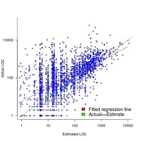
The fitted red line, for lines of code, shows the pattern commonly seen with effort estimation, i.e., underestimating small values and over estimating large values; but there is a much wider spread of actuals, and the cross-over point is much further up (if estimates below 50-lines are excluded, the exponent increases to 0.92, and the intercept decreases to 2, and the line shifts a bit.). The vertical river of actuals either side of the 10-LOC estimate looks very odd (estimating such small values happen when people estimate everything).
My article pointing out that software effort estimation is mostly fake research has been widely read (it appears in the first three results returned by a Google search on software fake research). The early researchers did some real research to build these models, but later researchers have been blindly following the early ‘prophets’ (i.e., later research is fake).
Lines of code probably does have an impact on effort, but estimating lines of code is a fool’s errand, and plugging estimates into models built from actuals is just crazy.
Pricing by quantity of source code
Software tool vendors have traditionally licensed their software on a per-seat basis, e.g., the cost increases with the number of concurrent users. Per-seat licensing works well when there is substantial user interaction, because the usage time is long enough for concurrent usage to build up. When a tool can be run non-interactively in the cloud, its use is effectively instantaneous. For instance, a tool that checks source code for suspicious constructs. Charging by lines of code processed is a pricing model used by some tool vendors.
Charging by lines of code processed creates an incentive to reduce the number of lines. This incentive was once very common, when screens supporting 24 lines of 80 characters were considered a luxury, or the BASIC interpreter limited programs to 1023 lines, or a hobby computer used a TV for its screen (a ‘tiny’ CRT screen, not a big flat one).
It’s easy enough to splice adjacent lines together, and halve the cost. Well, ease of splicing depends on programming language; various edge cases have to be handled (somebody is bound to write a tool that does a good job).
How does the tool vendor respond to a (potential) halving of their revenue?
Blindly splicing pairs of lines creates some easily detectable patterns in the generated source. In fact, some of these patterns are likely to be flagged as suspicious, e.g., if (x) a=1;b=2; (did the developer forget to bracket the two statements with { }).
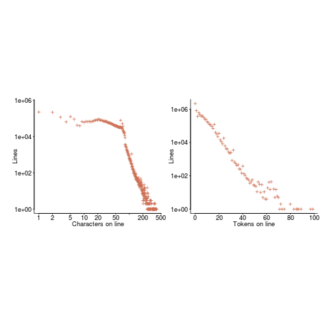
The plot below shows the number of lines in gcc 2.95 containing a given number of characters (left, including indentation), and the same count after even-numbered lines (with leading whitespace removed) have been appended to odd-numbered lines (code+data, this version of gcc was using in my C book):
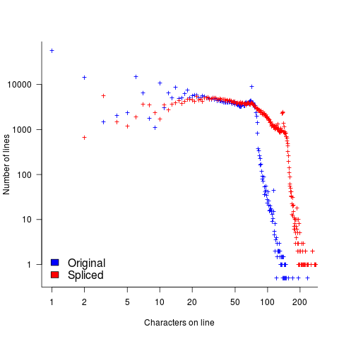
The obvious change is the introduction of a third straight’ish line segment (the increase in the offset of the sharp decline might be explained away as a consequence of developers using wider windows). By only slicing the ‘right’ pairs of lines together, the obvious patterns won’t be present.
Using lines of codes for pricing has the advantage of being easy to explain to management, the people who sign off the expense, who might not know much about source code. There are other metrics that are much harder for developers to game. Counting tokens is the obvious one, but has developer perception issues: Brackets, both round and curly. In the grand scheme of things, the use/non-use of brackets where they are optional has a minor impact on the token count, but brackets have an oversized presence in developer’s psyche.
Counting identifiers avoids the brackets issue, along with other developer perceptions associated with punctuation tokens, e.g., a null statement in an else arm.
If the amount charged is low enough, social pressure comes into play. Would you want to work for a company that penny pinches to save such a small amount of money?
As a former tool vendor, I’m strongly in favour of tool vendors making a healthy profit.
Creating an effective static analysis requires paying lots of attention to lots of details, which is very time-consuming. There are lots of not particularly good Open source tools out there; the implementers did all the interesting stuff, and then moved on. I know of several groups who got together to build tools for Java when it started to take-off in the mid-90s. When they went to market, they quickly found out that Java developers expected their tools to be free, and would not pay for claimed better versions. By making good enough Java tools freely available, Sun killed the commercial market for sales of Java tools (some companies used their own tools as a unique component of their consulting or service offerings).
Could vendors charge by the number of problems found in the code? This would create an incentive for them to report trivial issues, or be overly pessimistic about flagging issues that could occur (rather than will occur).
Why try selling a tool, why not offer a service selling issues found in code?
Back in the day a living could be made by offering a go-faster service, i.e., turn up at a company and reduce the usage cost of a company’s applications, or reducing the turn-around time (e.g., getting the daily management numbers to appear in less than 24-hours). This was back when mainframes ruled the computing world, and usage costs could be eye-watering.
Some companies offer bug-bounties to the first person reporting a serious vulnerability. These public offers are only viable when the source is publicly available.
There are companies who offer a code review service. Having people review code is very expensive; tools are good at finding certain kinds of problem, and investing in tools makes sense for companies looking to reduce review turn-around time, along with checking for more issues.
Impact of function size on number of reported faults
Are longer functions more likely to contain more coding mistakes than shorter functions?
Well, yes. Longer functions contain more code, and the more code developers write the more mistakes they are likely to make.
But wait, the evidence shows that most reported faults occur in short functions.
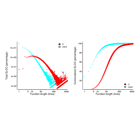
This is true, at least in Java. It is also true that most of a Java program’s code appears in short methods (in C 50% of the code is contained in functions containing 114 or fewer lines, while in Java 50% of code is contained in methods containing 4 or fewer lines). It is to be expected that most reported faults appear in short functions. The plot below shows, left: the percentage of code contained in functions/methods containing a given number of lines, and right: the cumulative percentage of lines contained in functions/methods containing less than a given number of lines (code+data):
Does percentage of program source really explain all those reported faults in short methods/functions? Or are shorter functions more likely to contain more coding mistakes per line of code, than longer functions?
Reported faults per line of code is often referred to as: defect density.
If defect density was independent of function length, the plot of reported faults against function length (in lines of code) would be horizontal; red line below. If every function contained the same number of reported faults, the plotted line would have the form of the blue line below.
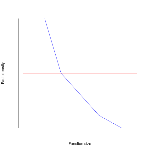
Two things need to occur for a fault to be experienced. A mistake has to appear in the code, and the code has to be executed with the ‘right’ input values.
Code that is never executed will never result in any fault reports.
In a function containing 100 lines of executable source code, say, 30 lines are rarely executed, they will not contribute as much to the final total number of reported faults as the other 70 lines.
How does the average percentage of executed LOC, in a function, vary with its length? I have been rummaging around looking for data to help answer this question, but so far without any luck (the llvm code coverage report is over all tests, rather than per test case). Pointers to such data very welcome.
Statement execution is controlled by if-statements, and around 17% of C source statements are if-statements. For functions containing between 1 and 10 executable statements, the percentage that don’t contain an if-statement is expected to be, respectively: 83, 69, 57, 47, 39, 33, 27, 23, 19, 16. Statements contained in shorter functions are more likely to be executed, providing more opportunities for any mistakes they contain to be triggered, generating a fault experience.
Longer functions contain more dependencies between the statements within the body, than shorter functions (I don’t have any data showing how much more). Dependencies create opportunities for making mistakes (there is data showing dependencies between files and classes is a source of mistakes).
The previous analysis makes a large assumption, that the mistake generating a fault experience is contained in one function. This is true for 70% of reported faults (in AspectJ).
What is the distribution of reported faults against function/method size? I don’t have this data (pointers to such data very welcome).
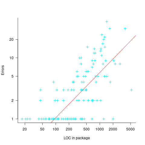
The plot below shows number of reported faults in C++ classes (not methods) containing a given number of lines (from a paper by Koru, Eman and Mathew; code+data):
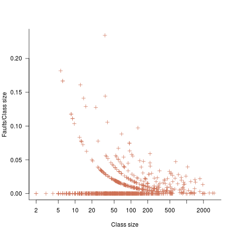
It’s tempting to think that those three curved lines are each classes containing the same number of methods.
What is the conclusion? There is one good reason why shorter functions should have more reported faults, and another good’ish reason why longer functions should have more reported faults. Perhaps length is not important. We need more data before an answer is possible.
How are C functions different from Java methods?
According to the right plot below, most of the code in a C program resides in functions containing between 5-25 lines, while most of the code in Java programs resides in methods containing one line (code+data; data kindly supplied by Davy Landman):
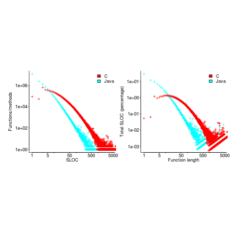
The left plot shows the number of functions/methods containing a given number of lines, the right plot shows the total number of lines (as a percentage of all lines measured) contained in functions/methods of a given length (6.3 million functions and 17.6 million methods).
Perhaps all those 1-line Java methods are really complicated. In C, most lines contain a few tokens, as seen below (code+data):
I don’t have any characters/tokens per line data for Java.
Is Java code mostly getters and setters?
I wonder what pattern C++ will follow, i.e., C-like, Java-like, or something else? If you have data for other languages, please send me a copy.
Plotting artifacts when the axis involves lines of code
While reading a report from the very late Rome period, the plot below caught my attention (the regression line was not in the original plot). The points follow a general trend, suggesting that when implementing a module, lines of code written per man-hour increases as the size of the module increases (in LOC). There are explanations for such behavior: perhaps module implementation time is mostly think-time that is independent of LOC, or perhaps larger modules contain more lines that can be quickly implemented (code+data).
Then I realised that the pattern of points was generated by a mathematical artifact. Can you spot the artifact?

The x-axis shows LOC, and the y-axis shows LOC/man-hour. Just plotting LOC against LOC would produce a row of points along a straight line, and if we treat dividing by man-hours as roughly equivalent to dividing by a random number (which might have some correlation with LOC), the result is points scattered around a line going up to the right.
If LOC-per-hour were constant, the points would form a horizontal line across the plot.
In the below left plot, from a different report (whose axis are function-points, and function-points implemented per month), the author has fitted a line, and it is close to horizontal (suggesting that the mean FP-per-month is constant).
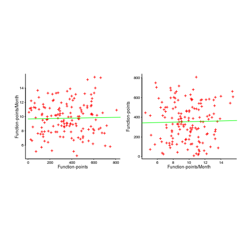
In fact the points are essentially random, and the line is a terrible fit (just how terrible is shown by switching the axis and refitting the line, above right; the refitted line should be vertical, but is horizontal. There is no connection between FP and FP-per-month, which is a good thing because the creators of function-points intended this to be true).
What process might generate this random scattering, rather than the trend seen in the first plot? If the implementation time was proportional to both the number of FP and some uniform random component, then the FP/time ratio would have the pattern seen.
The plots below show module size (in LOC) against man-hour (left) and FP against months (right):
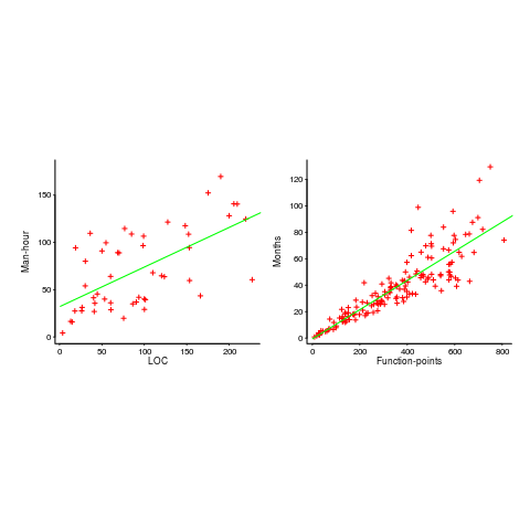
The module-LOC points are all over the place, while the FP points look as-if they are roughly consistent. Perhaps the module-LOC measurements came from a wide variety of sources, and we should not expect a visually pleasant trend.
Plotting LOC against LOC appears in other guises. Perhaps the most common being plotting fault-density against LOC; fault-density is generally calculated as faults/LOC.
Of course the artifacts also occur when plotting other kinds of measurements. Lines of code happens to be a commonly plotted quantity (at least in software engineering).
Growth of conditional complexity with file size
Conditional statements are a fundamental constituent of programs. Conditions are driven by the requirements of the problem being solved, e.g., if the water level is below the minimum, then add more water. As the problem being solved gets more complicated, dependencies between subproblems grow, requiring an increasing number of situations to be checked.
A condition contains one or more clauses, e.g., a single clause in: if (a==1), and two clauses in: if ((x==y) && (z==3)); a condition also appears as the termination test in a for-loop.
How many conditions containing one clause will a 10,000 line program contain? What will be the distribution of the number of clauses in conditions?
A while back I read a paper studying this problem (“What to expect of predicates: An empirical analysis of predicates in real world programs”; Google currently not finding a copy online, grrr, you will have to hassle the first author: durelli@icmc.usp.br, or perhaps it will get added to a list of favorite publications {be nice, they did publish some very interesting data}) it contained a table of numbers and yesterday my analysis of the data revealed a surprising pattern.
The data consists of SLOC, number of files and number of conditions containing a given number of clauses, for 63 Java programs. The following plot shows percentage of conditionals containing a given number of clauses (code+data):
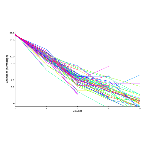
The fitted equation, for the number of conditionals containing a given number of clauses, is:

where:  (the coefficient for the fitted regression model is 0.56, but square-root is easier to remember),
  , and
, and  is the number of clauses.
The fitted regression model is not as good when  or
or  is always used.
This equation is an emergent property of the code; simply merging files to increase the average length will not change the distribution of clauses in conditionals.
When  , all conditionals contain the same number of clauses, off to infinity. For the 63 Java programs, the mean was 2,625, maximum 11,710, and minimum 172.
I was expecting SLOC to have an impact, but was not expecting number of files to be involved.
What grows with SLOC? Number of global variables and number of dependencies. There are more things available to be checked in larger programs, and an increase in dependencies creates the need to perform more checks. Also, larger programs are likely to contain more special cases, which are likely to involve checking both general and specific values (i.e., more clauses in conditionals); ok, this second sentence is a bit more arm-wavy than the first. The prediction here is that the percentage of global variables appearing in conditions increases with SLOC.
Chopping stuff up into separate files has a moderating effect. Since I did not expect this, I don’t have much else to say.
This model explains 74% of the variance in the data (impressive, if I say so myself). What other factors might be involved? Depth of nesting would be my top candidate.
Removing non-if-statement related conditionals from the count would help clarify things (I don’t expect loop-controlling conditions to be related to amount of code).
Two interesting data-sets in one week, with 10-days still to go until Christmas 🙂
Update: Fitting the same equation to the data from a later paper by the same group, based on mobile applications written in Swift and Objective-C, also produces a well-fitted regression model (apart from the term specifying an interactions between and  ).
).
Update: Thanks to Frank Busse for reminding me of the FAA report An Investigation of Three Forms of the Modified Condition Decision Coverage (MCDC) Criterion, which contains detailed information on the 20,256 conditionals in five Ada programs. The number of conditionals containing a given number of clauses is fitted by a power law (exponent is approximately -3).
Recent Comments