Archive
Number of calls to/from functions vs function length
Depending on the language the largest unit of code is either a sequence of statements contained in a function/procedure/subroutine or a set of functions/methods contained in a larger unit, e.g., class/module/file. Connections between these largest units (e.g., calls to functions) provide a mechanism for analysing the structure of a program. These connections form a graph, and the structure is known as a call graph.
It is not always possible to build a completely accurate call graph by analysing a program’s source code (i.e., a static call graph) when the code makes use of function pointers. Uncertainty about which functions are called at certain points in the code is a problem for compiler writers wanting to do interprocedural flow analysis for code optimization, and static analysis tools looking for possible coding mistakes.
The following analysis investigates two patterns in the function call graph of C/C++ programs. While calls via function pointers can be very common at runtime, they are uncommon in the source. Function call information was extracted from 98 GitHub projects using CodeQL.
Functions that contain more code are likely to contain more function calls. The plot below shows lines of code against number of function calls for each of the 259,939 functions in whatever version of the Linux kernel is on GitHub today (25 Jan 2026), the red line is a regression fit showing  (the fit systematically deviates for larger functions {yet to find out why}; code and data):
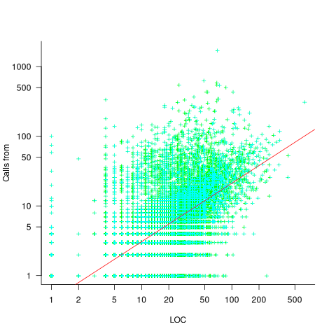
Researchers sometimes make a fuss of the fact that the number of calls per function is a power law, failing to note that this power law is a consequence of the number of lines per function being a power law (with an exponent of 2.8 for C, 2.7 for Java and 2.6 for Pharo). There are many small functions containing a few calls and a few large functions containing many calls.
Are more frequently called functions smaller (perhaps because they perform a simple operation that often needs to be done)? Widely used functionality is often placed in the same source file, and is usually called from functions in other files. The plot below shows the size of functions (in line of code) and the number of calls to them, for the 259,939 functions in the Linux kernel, with lines showing a LOESS fit to the corresponding points (code and data):
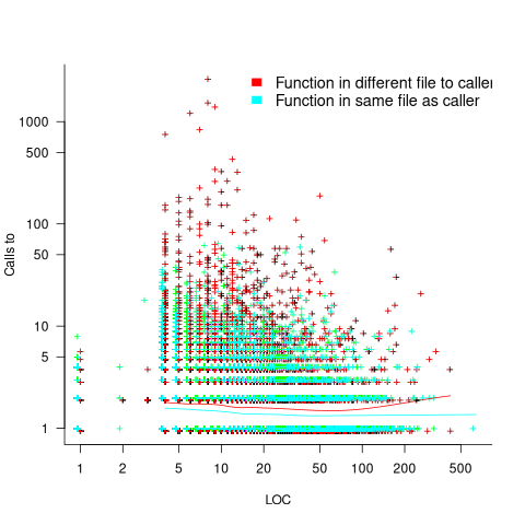
The apparent preponderance of red towards the upper left suggests that frequently called functions are short and contained in files different from the caller. However, the fitted LOESS lines show that the average difference is relatively small. There are many functions of a variety of sizes called once or twice, and few functions called very many times.
The program structure visible in a call graph is cluttered by lots of noise, such as calls to library functions, and the evolution baggage of previous structures. Also, a program may be built from source written in multiple languages (C/C++ is the classic example), and language interface issues can influence organization locally and globally (for instance, in Alibaba’s weex project the function main (in C) essentially just calls serverMain (in C++), which contains lots of code).
I suspect that many call graphs can be mapped to trees (the presence of recursion, though a chain of calls, sometimes comes as a surprise to developers working on a project). Call information needs to be integrated with loops and if-statements to figure out story structures (see section 6.9.1 of my C book). Don’t hold your breath for progress.
I expect that the above patterns are present in other languages. CodeQL supports multiple languages, but CodeQL source targeting one language has to be almost completely reworked to target another language, and it’s not always possible to extract exactly the same information. C/C++ appears have the best support.
Function calls are a component information
Lifetime of coding mistakes in the Linux kernel
What is the lifetime of coding mistakes in the Linux kernel? Some coding mistakes result in fault reports (some of which are fixed), while many are removed when the source that contains them is deleted/changed during ongoing development.
After fixing the coding mistake(s) in the kernel that generated a reported fault, developer(s) log the commit that introduced the coding mistake, along with the commit that fixed it. This logging started in 2013, and I only found out about it this week. To be exact, I discovered the repo: A dataset of Linux Kernel commits created by Maes Bermejo, Gonzalez-Barahona, Gallego, and Robles.
The log contains the commit hashes for the 90,760 fixes made to the 63 mainline kernel versions from 3.12 to 6.13. The complete log of 1,233,421 commits has to be searched to extract the details, e.g., date, lines added, etc.
The kernel development process involves regular release cycles of around 80 days. Developers submit the code they want to be included in the next release, this goes through a series of reviews, with Linus making the final decision.
The following analysis is based on the coding mistakes introduced between successive kernel releases, e.g., version 3.13 coding mistakes are those introduced into the source between 4 Nov 2013 (the day after version 3.12 was released) and 19 Jan 2014 (when version 3.13 was released). Code will have been worked on, and mistakes created/fixed, before it reached the kernel, which ensures some level of maturity.
The number of people working with pre-release code is likely to be tiny, compared to the number running released kernels. Consequently, the characteristics of coding mistake lifetime is expected to be different pre/post release, if only because more users are likely to report more faults.
The plot below shows the pre-release daily mistake fixed density against days since start of work on the current release, the red line is a fitted regression line mapped to density (fitted regression is a biexponential; code and data):
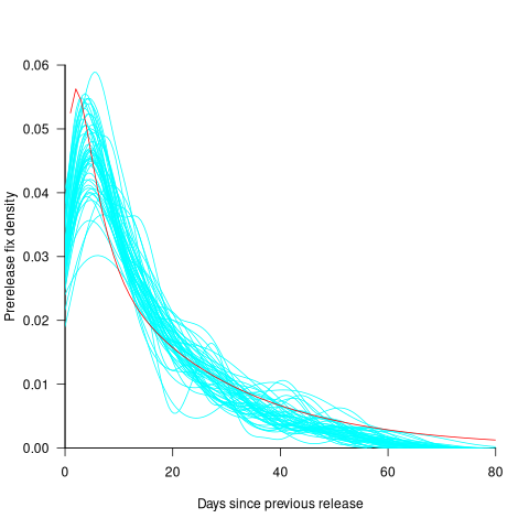
For all versions, the prior to release daily fix rate follows a consistent pattern: Most fixes occur in the first few days, with roughly an exponential decline to the release date.
The following analysis builds a broad brush model of cumulative fixes over time across 53 mainline kernel releases (the final 10 releases were not included because of their relatively short history).
The number of users of a new kernel takes time to increase as it percolates onto systems, e.g., adopted by Linux distributions and then installed by users, or installed by cloud providers. Eventually, code first included in a particular version will be running on most systems.
The post release daily fix rate is best modelled using the cumulative number of fixes, i.e., total number of fixes up to a given day since release. The models fitted below are based on dividing the post release cumulative fixes into before/after 200 days since release. The 200-day division is a round number (technically, a nearby value may provide a better fit) that supports the fitting of good quality before/after regression models. Averaged over all releases, 42% of fixes occurred within 200-days, and 58% after 200-days.
The plot below shows the cumulative number of post-release fixed faults, in red, for various kernel versions, with fitted regression lines in green and blue (grey line is at 200-days; code and data):

The equation fitted to the before 200-days fixes had the following form:
}")
where:  is a kernel version specific constant; see plot below.
The equation fitted to the after 200-days fixes had the following form:

where:  is a kernel version specific constant; see plot below.
Approximately, after release, the cumulative fix rate starts out quadratic in elapsed days, with the rate decreasing over time, until after 200-days the rate settles down to following the cube-root of days.
Comparing the number of post-release fixes across versions, there is a lot more variability in the first 200-days (i.e., the model fit to the data is sometimes very poor), relatively to after 200-days (where the model fit is consistently good).
Each kernel release has its own characteristics, parameterised by the values , and in the above equations. The plot below shows these values across versions, with red for , blue/green for , and grey line showing normalised LOC added/changed in the release (code and data):
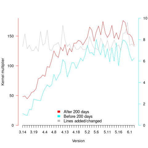
The plot clearly shows a large increase in the number of fixes between kernel version 3.14 and later versions. The before 200-days rate (blue/green) increase by a factor of seven, while the after 200-days rate increased by a factor of three.
Is this increase driven by some underlying factor in kernel development, or is it an external factor such as an increase in the number of users (more users leads to more faults reports), or the extensive post-release fuzz testing that is now common.
The number of lines of code added/changed, indicated by the grey line (shifted to fit plot axes) cannot be added to the fitted models because they exactly correlate with their respective version.
What is driving the long-term rate of fixes, i.e., cube-root of elapsed days?
Actually, what people are really want to know is what can be done to reduce the number of fixes required after release. When people ask me this, my usual reply is: “Spend more on testing”.
The probability of a coding mistake causing a fault report is decreasing: fixes reduce the number of remaining mistakes, and source added in one kernel version may be removed in a later version.
Perhaps the set of input behaviors is growing, producing the distinct conditions needed to trigger different coding mistakes, or the faults are occurring but are only reported when experienced by a small subset of users.
As always, more data is needed.
Update
Some data on Linux kernel use by AWS.
A safety-critical certification of the Linux kernel
This week there was an announcement on the system-safety mailing list that the Red Hat In-Vehicle Operating System (a version of the Linux kernel, plus a few subsystems) had been certified as being “… capable for use in ASIL B applications, …”. The Automotive Safety Integrity Levels (ASIL A is the lowest level, with D the highest; an example of ASIL B is controlling brake lights) are defined by ISO 26262, an international standard for functional safety of electrical and/or electronic systems installed in production road vehicles.
Given all I had heard about the problems that needed to be solved to get a safety certification for something as large and complicated as the Linux kernel, I wanted to know more about how Red Hat had achieved this certification.
The traditional, idealised, approach to certifying software is to check that all requirements are documented and traceable to the design, source code, tests, and test results. This information can be used to ensure that every requirement is implemented and produces the intended behavior, and that no undocumented functionality has been implemented.
When this approach is not practical (because of onerous time/cost), a potential get out of jail card is to use a Rigorous Development Process. Certification friendly development processes appear to revolve around lots of bureaucracy and following established buzzword techniques. The only development processes that have sometimes produced very reliable software all involve spending lots of time/money.
The major problems with certifying Linux are the apparent lack of specification/requirements documents, and a development process that does not claim to be rigorous.
The Red Hat approach is to treat the Linux man pages as the specification, extract the requirements from these pages, and then write the appropriate tests. Traceability looks like it is currently on the to-do list.
I have spent a lot of time working to understand specifications and their requirements; first with the C Standard and then with the Microsoft Server Protocols. This is the first time I have encountered man pages being used in a formal setting (sometimes they are used as one of the inputs to a reimplementation of a library).
Very little Open source software has a written specification in the traditional sense of a document cited in a contract that the vendor agrees to implement. Manuals, READMEs and help pages are not written in the formal style of a specification. A common refrain is that the source code is the specification. However, source is a specification of what the program does, it is not a specification of what the program is supposed to do.
The very nature of the Agile development process demands that there not be a complete specification. It’s possible that user stories could be treated as requirements.
There is an ISO Standard with Linux in its title: the Linux Base Standard. The goal of this Standard “… is to develop and promote a set of open standards that will increase compatibility among Linux distributions and enable software applications to run on any compliant system …”, i.e., it is not a specification of an OS kernel.
POSIX is a specification of the behavior of an OS (kernel functionality is specified by POSIX.1, .2 is shell and utilities, plus other .x documents). It’s many years since I tracked POSIX/Linux compliance, which was best described as “highly compatible”. Both Grok3 and ChatGPT o4 agree that “highly compatible” is still true, and list some known incompatibilities.
While they are not written in the form of a specification, the Linux man pages do have a consistent structure and are intended to be up-to-date. A person with a background of working with Linux kernels could probably extract meaningful requirements.
How many requirements are needed to cover the behavior of the Linux kernel?
On my computer running a 6.8.0-51 kernel, the /usr/include/linux directory contains 587 header files. Based on an analysis from 20 years ago (table 1897.1), most of these headers only declare macros and types (e.g., memory layout), not function declarations. The total number of function declarations in these headers is probably in the low thousands. POSIX (2008 version) defines 1,177 functions, but the number of system calls is probably around 300-400. Android implements 821 of these functions, of which 343 are system call related.
Let’s assume 2,000 functions. Some of these functions have an argument that specifies one or more optional values, each specifying a different sub-behavior. How many different sub-behaviors are there? If we assume that each kind of behavior is specified using a C macro, then Table 1897.1 suggests there might be around 10k C macros defined in these headers.
With positive/negative tests for each case, in round numbers we get (ignoring explicit testing of the values of struct members): *2 = 24,000") test files.
test files.
This calculation does not take into account combinations of options. I’m assuming that each test file will loop through various combinations of its kind of sub-behavior.
The 1990 C compiler validation suite contained around 1k tests. Thirty-five years later, 24k test files for a large OS feels low, but then combination testing should multiply the number of actual tests by at least an order of magnitude.
What is this hand-wavy analysis missing?
I suspect that the kernel is built with most of the optional functionality conditionally compiled out. This could significantly reduce the number of api functions and the supported options.
I have not taken into account any testing of the user-visible kernel data structures (because I don’t have any occurrence data).
Comments from readers with experience in testing OSes most welcome.
Another source of Linux specific information is the Linux Kernel documentation project. I don’t have any experience using this documentation, but the API documentation is very minimalist (automatically extracted from the source; the Assessment report lists this document as [D124], but never references it in the text).
Readers familiar with safety standards will be asking about the context in which this certification applies. Safety functions are not generic; they are specific to a safety-related system, i.e., software+hardware. This particular certification is for a Safety Element out of Context (SEooC), where “out of context” here means without the context of a system or knowledge of the safety goals. SEooC supports a bottom up approach to safety development, i.e., Safety Elements can be combined, along with the appropriate analysis and testing, to create a safety-related system.
This certification is the first of what I think will be many certifications of Linux, some at more rigorous safety levels.
if statement conditions, some basic measurements
The conditions contained in if-statements control all the decisions a program makes, yet relatively little is known about their characteristics.
A condition contains one or more clauses, for instance, the condition (a && b) contains two clauses that both need to be true, for the condition to be true. An earlier post modelled the number of clauses in Java conditions, and found an exponential decline (around 90% of conditions contained a single clause, for C this is around 85%).
The condition in a nested if-statement contains implicit decisions, because its evaluation depends on the conditions evaluated by its outer if-statements. I have long predicted that, on average, the number of clauses in a condition will decrease as if-statement nesting increases, because some decisions are subsumed by outer conditions. I have not seen any measurements on conditionals vs nesting, and this week this question reached the top of my to-do list.
I used Coccinelle to extract the text contained in each condition, along with the start/end line numbers of the associated if/else compound statement(s). After almost 20 years, Coccinelle is still the most flexible C source analysis tool available that does not require delving into compiler internals. The following is an example of the output (code and data):
file;stmt;if_line;if_col;cmpd_end;cmpd_line_end;expr sqlite-src-3460100/src/fkey.c;if;240;10;240;243;aiCol sqlite-src-3460100/src/fkey.c;if;217;6;217;217;! zKey sqlite-src-3460100/src/fkey.c;if;275;8;275;275;i == nCol sqlite-src-3460100/src/fkey.c;if;1428;6;1428;1433;aChange == 0 || fkParentIsModified ( pTab , pFKey , aChange , bChngRowid ) sqlite-src-3460100/src/fkey.c;if;808;4;808;808;iChildKey == pTab -> iPKey && bChngRowid sqlite-src-3460100/src/fkey.c;if;452;4;452;454;nIncr > 0 && pFKey -> isDeferred == 0 |
The conditional expressions (last column above) were reduced to a basic form involving simple variables and logical operators, along with operator counts. Some example output below (code and data):
simp_expr,land,lor,ternary v1,0,0,0 v1 && v2,1,0,0 v1 || v2,0,1,0 v1 && v2 && v3,2,0,0 v1 || ( v2 && v3 ),1,1,0 ( v1 && v2 ) || ( v3 && v4 ),2,1,0 ( v1 ? dm1 : dm2 ),0,0,1 |
The C source code projects measured were the latest stable versions of Vim (44,205 if-statements), SQLite (27,556 if-statements), and the Linux kernel (version 6.11.1; 1,446,872 if-statements).
A side note: I was surprised to see the ternary operator appearing in some conditions; in effect, an if within an if (see last line of the previous example). The ternary operator usually appears as a component of a large conditional expression (e.g., x + ( v1 ? dm1 : dm2 ) > y), rather than itself containing clauses, e.g., ( v1 ? dm1 : dm2 ) && v2. I have not seen the requirements for this operator discussed in any analysis of MC/DC.
The plot below shows the number of if-statements occurring at a given nesting level, along with regression fits, of the form  , to the Vim and SQLite data; the Linux data was better fit by a power law (code+data):
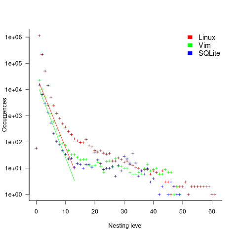
I suspect that most of the deeply nested levels in Vim and SQLite are the results of long else if chains, which, while technically highly nested, could all have been written having the same nesting level, such as the following:
if (strcmp(x, "abc")) ; // code else if (strcmp(x, "xyz")) ; // code else if (strcmp(x, "123")) ; // code |
This if else pattern does not appear to be common in Linux. Perhaps ‘regularizing’ the if else sequences in Vim and SQLite will move the distribution towards a power law (i.e., like Linux).
Average nesting depth will also be affected by the average number of lines per function, with functions containing more statements providing the opportunity for more deeply nested if-statements (rather than calling a function containing nested if-statements).
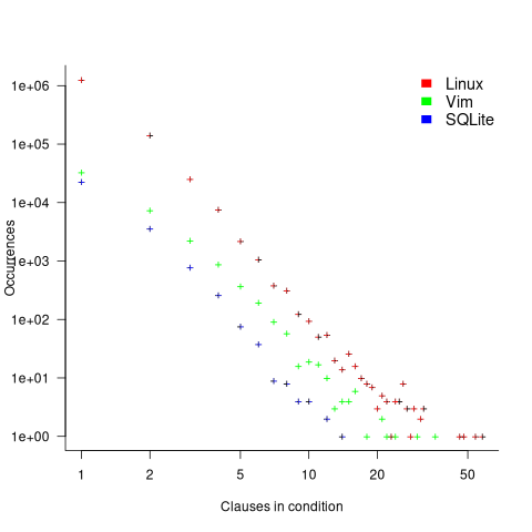
The plot below shows the number of occurrences of conditions containing a given number of clauses. Neither the exponential and power law are good fits, and log-log axis are used because it shows the points are closer to forming a straight line (code+data):
The plot below shows the nesting level and number of clauses in the condition for each of the 1,446,872 if-statements in the Linux kernel. Each value was ‘jittered’ to distribute points about their actual value, creating a more informative visualization (code+data):
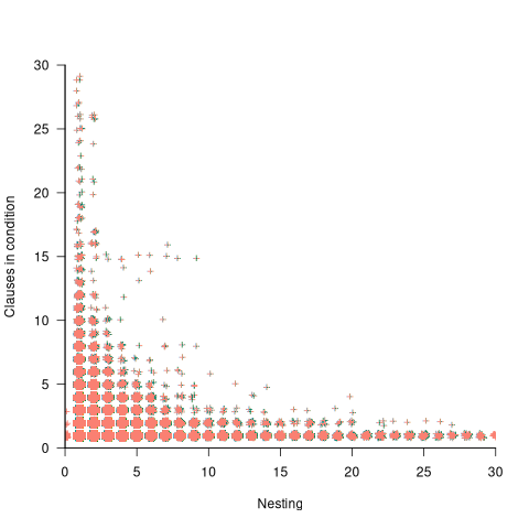
As expected, the likelihood of a condition containing multiple clauses does decrease with nesting level. However, with around 85% of conditions containing a single clause, the fitted regression models essential predict one clause for all nesting levels.
Measuring non-determinism in the Linux kernel
Developers often assume that it’s possible to predict the execution path a program will take, for a given set of input values, i.e., program behavior is deterministic. The execution path may be very complicated, and may depend on the contents of certain files (e.g., SQL engines), but it’s deterministic.
There is one kind of program where determinism is not an option; operating systems are non-deterministic when running in a mode where interrupts can occur.
How much non-determinism can occur in, say, Linux? For instance, when a program calls a system function (e.g., open, read, write, close), how often does the execution sequence follow the function call tree that appears in the source code, and how many different call sequences actually occur during program execution (because of diversions caused by an interrupt; ignoring control flow within functions)?
A study by Imanol Allende ran the same program 500K+ times, and traced every function call that occurred within the Linux kernel (thanks to Imanol for sending me the data and answering my questions). The program used appears below; the system calls traced were open (two distinct calls), read, write, and close (two distinct calls); a total of six system calls.
// #includes omitted int main(int argc, char **argv) { unsigned char result; int fd1, fd2, ret; char res_str[10]={0}; fd1 = open("/dev/urandom", O_RDONLY); fd2 = open("/dev/null", O_WRONLY); ret = read(fd1 , &result, 1); sprintf(res_str ,"%d", result); ret = write(fd2, res_str, strlen(res_str)); close(fd1); close(fd2); return ret; } |
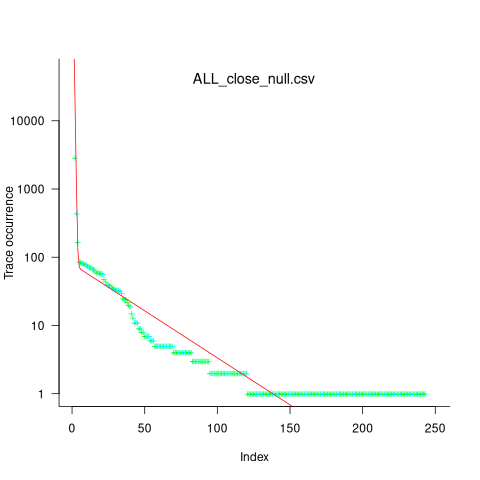
Analysing each of these six distinct calls, in around 98% of program runs, each call follows the same sequence of function calls within the kernel (the common case for write involves a chain of around 10 function calls). During the other 2’ish% of calls, the common sequence was interrupted for some reason, and the logged call trace includes additional called functions, e.g., calls involving the Read, Copy, Update synchronization mechanism. The plot below shows the growth in the number of unique traces against the number of program runs (436,827 of them) for the close(fd2) call; a fitted regression line is in red, with the first 1,000 runs not included in the fit (code+data):
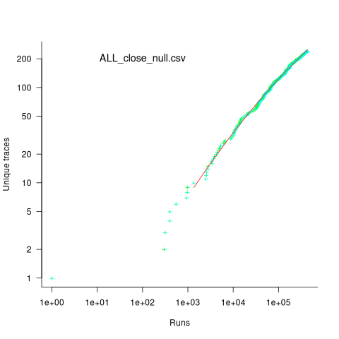
The fitted regression model is ^2") , suggesting that the growth in unique traces is slowing (this equation peaks at around
, suggesting that the growth in unique traces is slowing (this equation peaks at around  ), while the model fitted to some of the system calls implies ever continuing growth.
Allende investigated more sophisticated techniques for estimating the total number of unique traces, including: extreme value theory and species estimation techniques from ecology.
While around 98% of traces are the common case, over half of the unique traces occurred once in 436,827 runs. The plot below shows the number of occurrences of each unique trace, for the close(fd2) call, with an attempted fit of a bi-exponential model (in red; code+data):
The analysis above looked at one system call, the program contains six system calls. If, for each system call, the probability of the most common trace is 98%, then the probability of all six calls following their respective common case is 89%. As the number of distinct system calls made by a program goes up, the global common case becomes less common, and the number of distinct program traces increases multiplicatively.
Survival of CVEs in the Linux kernel
Software contained in safety related applications has to have a very low probability of failure.
How is a failure rate for software calculated?
The people who calculate these probabilities, or at least claim that some program has a suitably low probability, don’t publish the details or make their data publicly available.
People have been talking about using Linux in safety critical applications for over a decade (multiple safety levels are available to choose from). Estimating a reliability for the Linux kernel is a huge undertaking. This post is taking a first step via a broad brush analysis of a reliability associated dataset.
Public fault report logs are a very messy data source that needs a lot of cleaning; they don’t just contain problems caused by coding mistakes, around 50% are requests for enhancement (and then there is the issue of multiple reports having the same root cause).
CVE number are a curated collection of a particular kind of fault, i.e., information-security vulnerabilities. Data on 2,860 kernel CVEs is available. The data includes the first released version of the kernel containing the problem, and the version of the fixed release. The plot below shows the survival curve for kernel CVEs, with confidence intervals in blue/green (code+data):
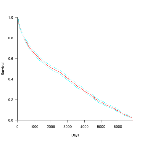
The survival curve appears to have two parts: the steeper decline during the first 1,000 days, followed by a slower, constant decline out to 16+ years.
Some good news is that many of these CVEs are likely to be in components that would not be installed in a safety critical application.
Predicting the size of the Linux kernel binary
How big is the binary for the Linux kernel? Depending on the value of around 15,000 configuration options, the size of the version 5.8 binary could be anywhere between 7.3Mb and 2,134 Mb.
Who is interested in the size of the Linux kernel binary?
We are not in the early 1980s, when memory for a desktop microcomputer often topped out at 64K, and software was distributed on 360K floppies (720K when double density arrived; my companies first product was a code optimizer which reduced program size by around 10%).
While desktop systems usually have oodles of memory (disk and RAM), developers targeting embedded systems seek to reduce costs by minimizing storage requirements, security conscious organizations want to minimise the attack surface of the programs they run, and performance critical systems might want a kernel that fits within a processors’ L2/L3 cache.
When management want to maximise the functionality supported by a kernel within given hardware resource constraints, somebody gets the job of building kernels supporting various functionality to find out the size of the binaries.
At around 4+ minutes per kernel build, it’s going to take a lot of time (or cloud costs) to compare lots of options.
The paper Transfer Learning Across Variants and Versions: The Case of Linux Kernel Size by Martin, Acher, Pereira, Lesoil, Jézéquel, and Khelladi describes an attempt to build a predictive model for the size of the kernel binary. This paper includes an extensive list of references.
The author’s approach was to first obtain lots of kernel binary sizes by building lots of kernels using random permutations of on/off options (only on/off options were changed). Seven kernel versions between 4.13 and 5.8 were used, producing 243,323 size/option setting combinations (complete dataset). This data was used to train a machine learning model.
The accuracy of the predictions made by models trained on a single kernel version were accurate within that kernel version, but the accuracy of single version trained models dropped dramatically when used to predict the binary size of later kernel versions, e.g., a model trained on 4.13 had an accuracy of 5% MAPE predicting 4.13, when predicting 4.15 the accuracy is 20%, and 32% accurate predicting 5.7.
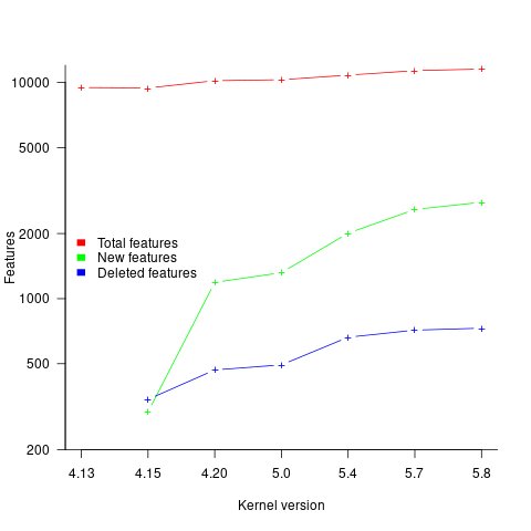
I think that the authors’ attempt to use this data to build a model that is accurate across versions is doomed to failure. The rate of change of kernel features (whose conditional compilation is supported by one or more build options) supported by Linux is too high to be accurately modelled based purely on information of past binary sizes/options. The plot below shows the total number of features, newly added, and deleted features in the modelled version of the kernel (code+data):
What is the range of impacts of each build option, on binary size?
If each build option is independent of the others (around 44% of conditional compilation directives in the kernel source contain one option), then the fitted coefficients of a simple regression model gives the build size increment when the corresponding option is enabled. After several cpu hours, the 92,562 builds involving 9,469 options in the version 4.13 build data were fitted. The plot below shows a sorted list of the size contribution of each option; the model  is 0.72, i.e., quite a good fit (code+data):

While the mean size increment for an enabled option is 75K, around 40% of enabled options decreases the size of the kernel binary. Modelling pairs of options (around 38% of conditional compilation directives in the kernel source contain two options) will have some impact on the pattern of behavior seen in the plot, but given the quality of the current model ( is 0.72) the change is unlikely to be dramatic. However, the simplistic approach of regression fitting the 90 million pairs of option interactions is not practical.
What might be a practical way of estimating binary size for any kernel version?
The size of a binary is essentially the quantity of code+static data it contains.
An estimate of the quantity of conditionally compiled source code dependent on a given option is likely to be a good proxy for that option’s incremental impact on binary size.
It’s trivial to scan source code for occurrences of options in conditional compilation directives, and with a bit more work, the number of lines controlled by the directive can be counted.
There has been a lot of evidence-based research on software product lines, and feature macros in particular. I was expecting to find a dataset listing the amount of code controlled by build options in Linux, but the data I can find does not measure Linux.
The Martin et al. build data is perfectfor creating a model linking quantity of conditionally compiled source code to change of binary size.
Analysis of a subset of the Linux Counter data
The Linux Counter project was started in 1993, with the aim of tracking the growth of Linux users (the kernel was first released two years earlier). Anybody could register any of their machines running Linux; a user ran a script that gathered basic information about a machine, and the output was emailed to the project. Once registered, users received an annual reminder to update information in their entry (despite using Linux since before the 1.0 release, user #46406 didn’t register until 2001).
When it closed (reopened/closed/coming back) it had 120K+ registered users. That’s a lot of information about computers, which unfortunately is not publicly available. I have not had any replies to my emails to those involved, asking for a copy that could be released in anonymized form.
This week I found 15,906 rows of what looks like a subset of the Linux counter data, most entries are post-2005. What did I learn from this data?
An obvious use is the pattern to check is changes over time. While the data does not include any explicit date, it does include the Kernel version, from which the earliest date can be inferred.
An earlier post used SPEC data to estimate the growth in installed memory over time; it has been doubling every 840 days, give or take. That data contains one data point per distinct vendor computer; the Linux counter data contains one entry per computer in use. There is around thirty pairs of entries for updated systems, i.e., a user updated the entry for an existing system.
The plot below shows memory installed in each registered computer, over time, for servers, laptops and workstations, with fitted regression lines. The memory size doubling times are: servers 4,000 days, laptops 2,000 days, and workstations 1,300 days (code+data):
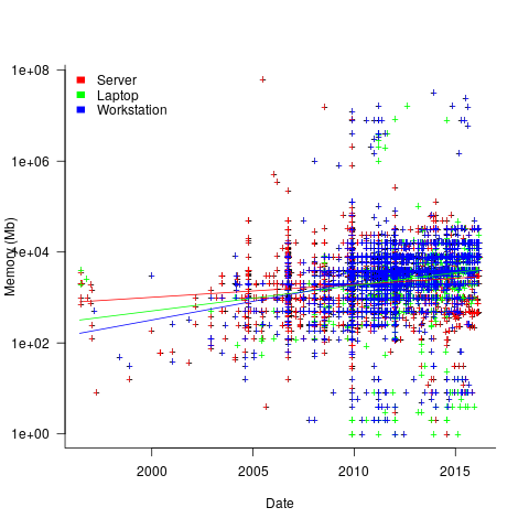
A regression model using dates is a good fit in the statistical sense, but explain very little of the variance in the data. The actual date on which the memory size was selected may have been earlier (because the kernel has been updated to a later release), or later (because memory was added, but the kernel was not updated).
Why is the memory doubling time so long?
Has memory size now reached the big-enough boundary, do Linux counter users keep the same system for many years without upgrading, are Linux counter systems retired Windows boxes that have been repurposed (data on installed memory Windows boxes would answer this point)?
Suggestions welcome.
When memory capacity is limited, it may be useful to swap least recently used memory contents to disc; Linux setup includes the specification of a swap partition. What is the optimal size of the size partition? A common recommendation is: if memory is less than 2G swap size is twice memory; if between 2-8G swap size is the same as memory, and for greater than 8G, half of memory size. The table below shows the percentage of particular system classes having a given swap/memory ratio (rounding the list of ratios to contain one decimal digit produces a list of over 100 ratio values).
swap/memory Server Workstation Laptop 1.0 15.2 19.9 25.9 2.0 10.3 9.6 8.6 0.5 9.5 7.7 8.4 |
The plot below shows memory against swap partition size, for the system classes laptop, server and workstation, with fitted regression line (code+data):
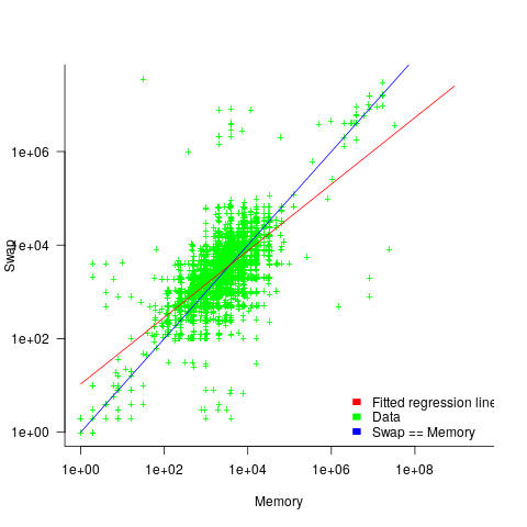
The available disk space also has a (small) impact on swap partition size; the following model explains 46% of the variance in the data:  .
.
I was hoping to confirm the rate of installed memory growth suggested by the SPEC data, with installed systems lagging a few years behind the latest releases. This Linux counter data tells a very different growth story. Perhaps pre-2005 data will tell another story (I just need to find it).
I’m not sure if the swap/memory ratio analysis is of any use to systems people. It was something of a fishing expedition on my part.
Other counting projects have included the Ubuntu counter project, and Hardware for Linux which is still active and goes back to August 2014.
I’m interested in hearing about the availability of any other Linux counter data, or data from other computer counting projects.
Linux has a sleeper agent working as a core developer
The latest news from Wikileaks, that GCHQ, the UK’s signal intelligence agency, has a sleeper agent working as a trusted member of the Linux kernel core development team should not come as a surprise to anybody.
The Linux kernel is embedded as a core component inside many critical systems; the kind of systems that intelligence agencies and other organizations would like full access.
The open nature of Linux kernel development makes it very difficult to surreptitiously introduce a hidden vulnerability. A friendly gatekeeper on the core developer team is needed.
In the Open source world, trust is built up through years of dedicated work. Funding the right developer to spend many years doing solid work on the Linux kernel is a worthwhile investment. Such a person eventually reaches a position where the updates they claim to have scrutinized are accepted into the codebase without a second look.
The need for the agent to maintain plausible deniability requires an arm’s length approach, and the GCHQ team made a wise choice in targeting device drivers as cost-effective propagators of hidden weaknesses.
Writing a device driver requires the kinds of specific know-how that is not widely available. A device driver written by somebody new to the kernel world is not suspicious. The sleeper agent has deniability in that they did not write the code, they simply ‘failed’ to spot a well hidden vulnerability.
Lack of know-how means that the software for a new device is often created by cutting-and-pasting code from an existing driver for a similar chip set, i.e., once a vulnerability has been inserted it is likely to propagate.
Perhaps it’s my lack of knowledge of clandestine control of third-party computers, but the leak reveals the GCHQ team having an obsession with state machines controlled by pseudo random inputs.
With their background in code breaking, I appreciate that GCHQ have lots of expertise to throw at doing clever things with pseudo random numbers (other than introducing subtle flaws in public key encryption).
What about the possibility of introducing non-random patterns in randomised storage layout algorithms (he says, waving his clueless arms around)?
Which of the core developers is most likely to be the sleeper agent? His codename, Basil Brush, suggests somebody from the boomer generation, or perhaps reflects some personal characteristic; it might also be intended to distract.
What steps need to be taken to prevent more sleeper agents joining the Linux kernel development team?
Requiring developers to provide a record of their financial history (say, 10-years worth), before being accepted as a core developer, will rule out many capable people. Also, this approach does not filter out ideologically motivated developers.
The world may have to accept that intelligence agencies are the future of major funding for widely used Open source projects.
Update
Turns out the sleeper agent was working on xz.
Predicting the future with data+logistic regression
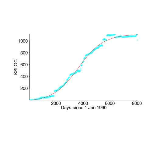
Predicting the peak of data fitted by a logistic equation is attracting a lot of attention at the moment. Let’s see how well we can predict the final size of a software system, in lines of code, using logistic regression (code+data).
First up is the size of the GNU C library. This is not really a good test, since the peak (or rather a peak) has been reached.
We need a system that has not yet reached an easily recognizable peak. The Linux kernel has been under development for many years, and lots of LOC counts are available. The plot below shows a logistic equation fitted to the kernel data, assuming that the only available data was up to day: 2,900, 3,650, 4,200, and 5,000+ (code+data). Can you tell which fitted line corresponds to which number of days?
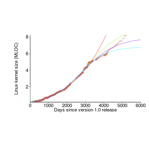
The underlying ‘problem’ is that we are telling the fitting software to fit a particular equation; the software does what it has been told to do, and fits a logistic equation (in this case).
A cubic polynomial is also a great fit to the existing kernel data (red line to the left of the blue line), and this fitted equation can be extended into future (to the right of the blue line); dotted lines are 95% confidence bounds. Do any readers believe the future size of the Linux kernel predicted by this cubic model?
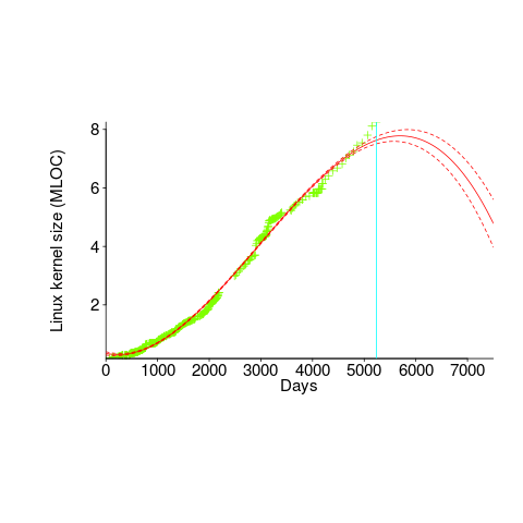
Predicting the future requires lots of data on the underlying processes that drive events. Modelling events is an iterative process. Build a model, check against reality, adjust model, rinse and repeat.
If the COVID-19 experience trains people to be suspicious of future predictions made by models, it will have done something positive.
Recent Comments