The Shape of Code

The SPEC benchmarks came out a year after the first release of gcc (in fact gcc was and still is one of the programs included in the benchmark). Compiling the SPEC programs using the gcc option -O2 (sometimes -O3) has always been the way to measure gcc performance, but after 25 years does this way of doing things tell us anything useful?

The short answer: No

The longer answer is below as another draft section from my book Empirical software engineering with R book. As always comments welcome.

Changes in optimization performance of gcc over time

The GNU Compiler Collection <book gcc-man_12> (GCC) is under active development with its most well known component, the C compiler gcc, now over 25 years old. After such a long period of development is the quality of code generated by gcc still improving and if so at what rate? The method typically used to measure compiler performance is to compile the [SPEC] benchmarks with a small set of optimization options switched on (e.g., the O2 or O3 options) and this approach is used for the analysis performed here.

Data

Vladimir N. Makarow measured the performance of 9 releases of gcc, occurring between 2003 and 2010, on the same computer using the same benchmark suite (SPEC2000); this data is used in the following analysis.

The data contains the [SPEC number] (i.e., runtime performance) and code size measurements on 12 integer programs (11 in C and one in C+\+) from SPEC2000 compiled with gcc versions 3.2.3, 3.3.6, 3.4.6, 4.0.4, 4.1.2, 4.2.4, 4.3.1, 4.4.0 and 4.5.0 at optimization levels O2 and O3 (the mtune=pentium4 option was also used) 32-bit for the Intel Pentium 4 processor.

The same integer programs and 14 floating-point programs (10 in Fortran and 4 in C) were compiled for 64-bits, again with the O2 and O3 options (the mpc64 floating-point option was also used), using gcc versions 4.0.4, 4.1.2, 4.2.4, 4.3.1, 4.4.0 and 4.5.0.

Is the data believable?

The following are two fitness-for-purpose issues associated with using programs from SPEC2000 for these measurements:

1. the benchmark is designed for measuring processor performance not
   compiler performance,
2. many of its programs have been used for compiler benchmarking for
   many years and it is likely that gcc has already been tuned to do
   well on this benchmark.

The runtime performance measurements were obtained by running each programs once, SPEC requires that each program be run three times and the middle one chosen. Multiple measurements of each program would have increased confidence in their accuracy.

Predictions made in advance

Developers continue to make improvements to gcc and it is hoped that its optimization performance is increasing, knowing that performance is at a steady state or decreasing performance is also of interest.

No hypothesis is proposed for how optimization performance, as measured by the O2 and O3 options, might change between releases of gcc over the period 2003 to 2010.

The gcc documentation says that using the O3 option causes more optimizations to be performed than when the O2 option is used and therefore we would expect better performance for programs compiled with O3.

Applicable techniques

Modelling individual O2 and O3 option performance
One technique for modelling changes in optimization performance is to build a linear model that fits the gcc version (i.e., version is the predictor variable) to the average performance of the code it generate, calculating the averaged performance over each of the programs measured with the corresponding version of gcc. The problem with this approach is that by calculating an average it is throwing away information that is available about the variation in performance across different programs.

Building a [mixed-effects] model would make use of all the data when fitting a relationship between two quantities where there is a recurring random component (i.e., the SPEC program used). The optimizations made are likely to vary between different SPEC programs, we could treat the performance variations caused by difference in optimization as being random and having an impact on the mean performance value of all programs.

Programs differ in the magnitude of their SPEC number and code size, the measurements were converted to the percentage change compared against the values obtained using the earliest version of gcc in the measurement set.

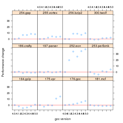
Figure 1. Percentage change in SPEC number (relative to version 4.0.4) for 12 programs compiled using 6 different versions of gcc (compiling to 64-bits with the O3 option).

Fitting a linear model requires at least two sets of [interval data]. The gcc version numbers are [ordinal values] and the following are two possible ways of mapping them to interval values:

1. there have been over 150 different released versions of gcc and a
   particular version could be mapped to its place in this sequence.
2. the date of release of a version can be mapped to the number of
   days since the first release.

If version releases are organized around new functionality added then it makes sense to use version sequence number. If the performance of a new optimization was proportional to the amount of effort (e.g., man days) that went into its implementation then it would make sense to use days between releases.

The versions tested by Makarow were each from a different secondary release within a given primary version line and at roughly yearly intervals (two years separated the first pair and one month another pair).

There have been approximately 25 secondary releases in the 25 year project and using a release version sequence number starting at 20 seems like a reasonable choice.

Internally a compiler optimizer performs many different kinds of optimizations (gcc has over 160 different options for controlling machine independent optimization behavior). While the implementation of a new optimization is a gradual process involving many days of work, from the external user perspective it either exists and does its job when a given optimization level is supported or it does not exist.

What is the shape of the performance/release-version relationship? In the first few years of a compilers development it is to be expected that all the known major (i.e., big impact) optimization will be implemented and thereafter newly added optimizations have a progressively smaller impact on overall performance. Given gcc’s maturity it looks reasonable to assume that new releases contain a few additional improvement that have an incremental impact, i.e., the performance/release-version relationship is assumed to be linear (no other relationship springs out of a plot of the data).

A mixed-effects model can be created by calling the R function lme from the package nlme. The only difference between the following call to lme and a call to lm is the third argument specifying the random component.

t.lme=lme(value ~ variable, data=lme.O2, random = ~ 1 | Name)

The argument random = ~ 1 | Name specifies that the random component effects the mean value of the result (when building a model this translates to an effect on the value of the intercept of the fitted equation) and that Name (of the program) is the grouped variable.

To specify that the random effect applies to the slope of the equation rather than its intercept the call is as follows:

t.lme=lme(value ~ variable, data=lme.O2, random = ~ variable -1 | Name)

To specify that both the slope and the intercept are effected the -1 is omitted (for this gcc data the calculation fails to converge when both can be effected).

Since the measurements are about different versions of gcc it is to be expected that the data format has a separate column for each version of gcc (the format that would be used to pass data lm) as follows:

      Name v3.2.3 v3.3.6 v3.4.6 v4.0.4 v4.1.2 v4.2.4 v4.3.1 v4.4.0 v4.5.0
1 164.gzip    933    932    957    922    933    939    917    969    955
2  175.vpr    562    561    577    576    586    585    576    589    588
3  176.gcc   1087   1084   1159   1135   1133   1102   1146   1189   1211

The relationship between the three variables in the call to lme is more complicated and the data needs to be reorganize so that one column contains all of the values, one the gcc version numbers and another column the program names. The function melt from package reshape2 can be used to restructure the data to look like:

          Name variable     value
11   256.bzip2   v3.2.3  0.000000
12   300.twolf   v3.2.3  0.000000
13 SPECint2000   v3.2.3  0.000000
14    164.gzip   v3.3.6 -0.107181
15     175.vpr   v3.3.6 -0.177936
16     176.gcc   v3.3.6 -0.275989
17     181.mcf   v3.3.6  0.148810

Comparing O2 and O3 option performance
When comparing two samples the [Wilcoxon signed-rank test] and the [Mann-Whitney U test] spring to mind. However, some of the expected characteristics of the data violate some of the properties that these tests assume hold (e.g., every release include new/updated optimizations which is likely to result in the performance of each release having a different mean and variance).

The difference in performance between the two optimization levels could be treated as a set of values that could be modelled using the same techniques applied above. If the resulting model have a line than ran parallel with the x-axis and was within the appropriate confidence bounds we could claim that there was no measurable difference between the two options.

Results

The following is the output produced by summary for a mixed-effect model, with the random variation assumed to effect the value of intercept, created from the SPEC numbers for the integer programs compiled for 64-bit code at optimization level O2:

Linear mixed-effects model fit by REML
 Data: lme.O2
       AIC      BIC    logLik
  453.4221 462.4161 -222.7111

Random effects:
 Formula: ~1 | Name
        (Intercept) Residual
StdDev:    7.075923 4.358671

Fixed effects: value ~ variable
                 Value Std.Error DF   t-value p-value
(Intercept) -29.746927  7.375398 59 -4.033264   2e-04
variable      1.412632  0.300777 59  4.696612   0e+00
 Correlation:
         (Intr)
variable -0.958

Standardized Within-Group Residuals:
        Min          Q1         Med          Q3         Max
-4.68930170 -0.45549280 -0.03469526  0.31439727  2.45898648

Number of Observations: 72
Number of Groups: 12

and the following summary output is from a linear model built from an average of the data used above.

Call:
lm(formula = value ~ variable, data = lmO2)

Residuals:
      13       26       39       52       65       78
 0.16961 -0.32719  0.47820 -0.47819 -0.01751  0.17508

Coefficients:
             Estimate Std. Error t value Pr(>|t|)
(Intercept) -28.29676    2.22483  -12.72 0.000220 ***
variable      1.33939    0.09442   14.19 0.000143 ***
---
Signif. codes:  0 ‘***’ 0.001 ‘**’ 0.01 ‘*’ 0.05 ‘.’ 0.1 ‘ ’ 1

Residual standard error: 0.395 on 4 degrees of freedom
Multiple R-squared: 0.9805,     Adjusted R-squared: 0.9756
F-statistic: 201.2 on 1 and 4 DF,  p-value: 0.0001434

The biggest difference is that the fitted values for the Intercept and slope (the column name, variable, gives this value) have a standard error that is 3+ times greater for the mixed-effects model compared to the linear model based on using average values (a similar result is obtained if the mixed-effects random variation is assumed to effect the slope and the calculation fails to converge if the variation is on both intercept and slope). One consequence of building a linear model based on averaged values is that some of the variations present in the data are smoothed out. The mixed-effects model is more accurate in that it takes all variations present in the data into account.

For integer programs compiled for 32-bits there is much less difference between the mixed-effects models and linear models than is seen for 64-bit code.

1. For SPEC performance the created models show:
   1. for the integer programs a rate of increase of around 0.6% (sd
      0.2) per release for O2 and O3 options on 32-bit code
      and an increase of 1.4% (sd 0.3) for 64-bit code,
   2. for floating-point, C programs only, a rate of increase per
      release of 12% (sd 5) at 32-bits and 1.4% (sd 0.7) at 64-bits, with
      very little difference between the O2 and O3 options.
2. For size of generated code the created models show:
   1. for integer programs 32-bit code built using O2 size is
      decreasing at the rate of 0.6% (sd 0.1) per release, while for both
      64-bit code and O3 the size is increasing at between 0.7% (sd
      0.2) and 2.5% (sd 0.4) per release,
   2. for floating-point, C programs only, 32-bit code built using
      O2 had an unacceptable p-value, while for both 64-bit code
      and O3 the size is increasing at between 1.6% (sd 0.3) and
      9.3 (sd 1.1) per release.

Comparing O2 and O3 option performance
The intercept and slope values for the models built for the SPEC integer performance difference had p-values way too large to be of interest (a ballpark estimate of the values would suggest very little performance difference between the two options).

The program size change models showed O3 increasing, relative to O2, at 1.4% to 1.7% per release.

Discussion

The average rate of increase in SPEC number is very low and does not appear to be worth bothering about, possible reasons for this include:

1. a lot of effort has already been invested in making sure that gcc
   performs well on the SPEC programs and the optimizations now being
   added to gcc are aimed at programs having other kinds of
   characteristics,
2. gcc is a mature compiler that has implemented all of the worthwhile
   optimizations and there are no more major improvements left to be
   made,
3. measurements based on just setting the O2 or O3
   options might not provide a reliable guide to gcc optimization
   performance. The command
   gcc -c -Q -O2 --help=optimizers
   shows that for gcc version 4.5.0 the O2 option enables 91 of
   the possible 174 optimization options and the O3 option
   enables 7 more. Performing some optimizations together sometimes
   results in poorer quality code than if a subset of those
   optimizations had been applied (genetic programming is being
   researched as one technique for selecting the best optimizations
   options to use for a given program and up to 13% improvements have
   been obtained over gcc’s -O options <book Bashkansky_07>). The
   percentage performance change figure above shows
   that for some programs performance decreases on some releases.

   Whole program optimization is a major optimization area that has been addressed in recent versions of gcc, this optimizations is not enabled by the O options.

The percentage differences in SPEC integer performance between the O2 and O3 options were very small, but varied too much to be able to build a reliable linear model from the values.

For SPEC program code size there is a significant different between the O2 and O3 options. This is probably explained by function inlining being one of the seven additional optimization enabled by O3 (inlining multiple calls to the same function often increases code size <book inlining> and changes to the inlining optimization over releases could result in more functions being inlined).

Conclusion

Either the optimizations added to gcc between 2003 and 2010 have not made any significant difference to the performance of the generated code or the established method of measuring gcc optimization performance (i.e., the SPEC benchmarks and the O2 or O3 compiler options) is no longer a reliable indicator.