Archive
Modelling time to next reported fault
After the arrival of a fault report for a program, what is the expected elapsed time until the next fault report arrives (assuming that the report relates to a coding mistake and is not a request for enhancement or something the user did wrong, and the number of active users remains the same and the program is not changed)? Here, elapsed time is a proxy for amount of program usage.
Measurements (here and here) show a consistent pattern in the elapsed time of duplicate reports of individual faults. Plotting the time elapsed between the first report and the n’th report of the same fault in the order they were reported produces an exponential line (there are often changes in the slope of this line). For example, the plot below shows 10 unique faults (different colors), the number of days between the first report and all subsequent reports of the same fault (plus character); note the log scale y-axis (discussed in this post; code+data):

The first person to report a fault may experience the same fault many times. However, they only get to submit one report. Also, some people may experience the fault and not submit a report.
If the first reporter had not submitted a report, then the time of first report would be later. Also, the time of first report could have been earlier, had somebody experienced it earlier and chosen to submit a report.
The subpopulation of users who both experience a fault and report it, decreases over time. An influx of new users is likely to cause a jump in the rate of submission of reports for previously reported faults.
It is possible to use the information on known reported faults to build a probability model for the elapsed time between the last reported known fault and the next reported known fault (time to next reported unknown fault is covered at the end of this post).
The arrival of reports for each distinct fault can be modelled as a Poisson process. The time between events in a Poisson process with rate  has an exponential distribution, with mean
  . The distribution of a sum of multiple Poisson processes is itself a Poisson process whose rate is the sum of the individual rates. The other key point is that this process is memoryless. That is, the elapsed time of any report has no impact on the elapsed time of any other report.
If there are  different faults whose fitted report time exponents are:
  ,
,  …
…  , then summing the Poisson rates,
  , gives the mean
  , for a probability model of the estimated time to next any-known fault report.
To summarise. Given enough duplicate reports for each fault, it’s possible to build a probability model for the time to next known fault.
In practice, people are often most interested in the time to the first report of a previous unreported fault.
tl;dr Modelling time to next previously unreported fault has an analytic solution that depends on variables whose values have to be approximately approximated.
The method used to build a probability model of reports of known fault can be used extended to build a probability model of first reports of currently unknown faults. To build this model, good enough values for the following quantities are needed:
- the number of unknown faults,
 , remaining in the program. I have some ideas about estimating the number of unknown faults, , and will discuss them in another post,
 - the time,
 , needed to have received at least one report for each of the unknown faults. In practice, this is the lifetime of the program, and there is data on software half-life. However, all coding mistakes could trigger a fault report, but not all coding mistakes will have done so during a program’s lifetime. This is a complication that needs some thought,
 - the values of
 ,
,  …
…  for each of the unknown faults. There is some data suggesting that these values are drawn from an exponential distribution, or something close to one. Also, an equation can be fitted to the values of the known faults. The analysis below assumes that the
  for each unknown fault that might be reported is randomly drawn from an exponential distribution whose mean is .
This rate will be affected by program usage (i.e., number of users and the activities they perform), and source code characteristics such as the number of executions paths that are dependent on rarely true conditions.
Putting it all together, the following is the question I asked various LLMs (which uses  , rather than ):
There are independent processes. Each process,  , transmits a signal, and the number of signals transmitted in a fixed time interval, , has a Poisson distribution with mean
  for
for  . The values are randomly drawn from the same exponential distribution. What is the cumulative distribution for the time between the successive first signals from the processes.
The cumulative distribution gives the probability that an event has occurred within a given amount of time, in this case the time since the last fault report.
The ChatGPT 5.2 Thinking response (Grok Thinking gives the same formula, but no chain of thought): The probability that the  unknown fault is reported within time
  of the previous report of an unknown fault,
 ") , is given by the following rather involved formula:
, is given by the following rather involved formula:
=1-(a/{a+t})^{N-k}{}_{2}F_1(N-k, k; N+1; t/{a+t})")
where: is the initial number of faults that have not been reported,  , and
, and  is the hypergeometric function.
The important points to note are: the value  decreases as more unknown faults are reported, and the dominant contribution of the value .
Deepseek’s response also makes complicated use of the same variables, and the analysis is very similar before making some simplifications that don’t look right (text of response). Kimi’s response is usually very good, but for this question failed to handle the consequences of .
Almost all published papers on fault prediction ignore the impact of number of users on reported faults, and that report time for each distinct fault has a distinct distribution, i.e., their analysis is not connected to reality.
Lifetime of coding mistakes in the Linux kernel
What is the lifetime of coding mistakes in the Linux kernel? Some coding mistakes result in fault reports (some of which are fixed), while many are removed when the source that contains them is deleted/changed during ongoing development.
After fixing the coding mistake(s) in the kernel that generated a reported fault, developer(s) log the commit that introduced the coding mistake, along with the commit that fixed it. This logging started in 2013, and I only found out about it this week. To be exact, I discovered the repo: A dataset of Linux Kernel commits created by Maes Bermejo, Gonzalez-Barahona, Gallego, and Robles.
The log contains the commit hashes for the 90,760 fixes made to the 63 mainline kernel versions from 3.12 to 6.13. The complete log of 1,233,421 commits has to be searched to extract the details, e.g., date, lines added, etc.
The kernel development process involves regular release cycles of around 80 days. Developers submit the code they want to be included in the next release, this goes through a series of reviews, with Linus making the final decision.
The following analysis is based on the coding mistakes introduced between successive kernel releases, e.g., version 3.13 coding mistakes are those introduced into the source between 4 Nov 2013 (the day after version 3.12 was released) and 19 Jan 2014 (when version 3.13 was released). Code will have been worked on, and mistakes created/fixed, before it reached the kernel, which ensures some level of maturity.
The number of people working with pre-release code is likely to be tiny, compared to the number running released kernels. Consequently, the characteristics of coding mistake lifetime is expected to be different pre/post release, if only because more users are likely to report more faults.
The plot below shows the pre-release daily mistake fixed density against days since start of work on the current release, the red line is a fitted regression line mapped to density (fitted regression is a biexponential; code and data):
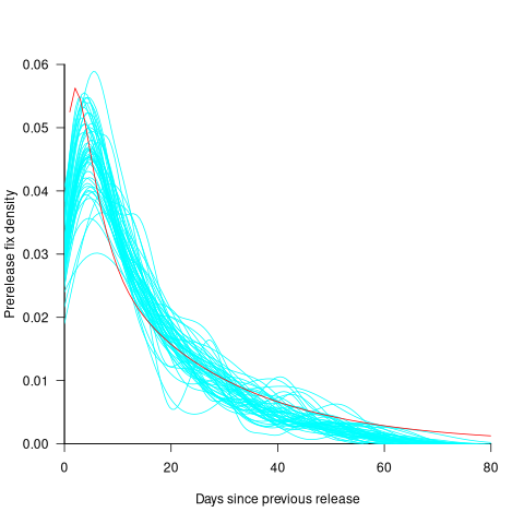
For all versions, the prior to release daily fix rate follows a consistent pattern: Most fixes occur in the first few days, with roughly an exponential decline to the release date.
The following analysis builds a broad brush model of cumulative fixes over time across 53 mainline kernel releases (the final 10 releases were not included because of their relatively short history).
The number of users of a new kernel takes time to increase as it percolates onto systems, e.g., adopted by Linux distributions and then installed by users, or installed by cloud providers. Eventually, code first included in a particular version will be running on most systems.
The post release daily fix rate is best modelled using the cumulative number of fixes, i.e., total number of fixes up to a given day since release. The models fitted below are based on dividing the post release cumulative fixes into before/after 200 days since release. The 200-day division is a round number (technically, a nearby value may provide a better fit) that supports the fitting of good quality before/after regression models. Averaged over all releases, 42% of fixes occurred within 200-days, and 58% after 200-days.
The plot below shows the cumulative number of post-release fixed faults, in red, for various kernel versions, with fitted regression lines in green and blue (grey line is at 200-days; code and data):

The equation fitted to the before 200-days fixes had the following form:
}")
where:  is a kernel version specific constant; see plot below.
The equation fitted to the after 200-days fixes had the following form:

where:  is a kernel version specific constant; see plot below.
Approximately, after release, the cumulative fix rate starts out quadratic in elapsed days, with the rate decreasing over time, until after 200-days the rate settles down to following the cube-root of days.
Comparing the number of post-release fixes across versions, there is a lot more variability in the first 200-days (i.e., the model fit to the data is sometimes very poor), relatively to after 200-days (where the model fit is consistently good).
Each kernel release has its own characteristics, parameterised by the values , and in the above equations. The plot below shows these values across versions, with red for , blue/green for , and grey line showing normalised LOC added/changed in the release (code and data):
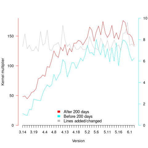
The plot clearly shows a large increase in the number of fixes between kernel version 3.14 and later versions. The before 200-days rate (blue/green) increase by a factor of seven, while the after 200-days rate increased by a factor of three.
Is this increase driven by some underlying factor in kernel development, or is it an external factor such as an increase in the number of users (more users leads to more faults reports), or the extensive post-release fuzz testing that is now common.
The number of lines of code added/changed, indicated by the grey line (shifted to fit plot axes) cannot be added to the fitted models because they exactly correlate with their respective version.
What is driving the long-term rate of fixes, i.e., cube-root of elapsed days?
Actually, what people are really want to know is what can be done to reduce the number of fixes required after release. When people ask me this, my usual reply is: “Spend more on testing”.
The probability of a coding mistake causing a fault report is decreasing: fixes reduce the number of remaining mistakes, and source added in one kernel version may be removed in a later version.
Perhaps the set of input behaviors is growing, producing the distinct conditions needed to trigger different coding mistakes, or the faults are occurring but are only reported when experienced by a small subset of users.
As always, more data is needed.
Update
Some data on Linux kernel use by AWS.
Half-life of Open source research software projects
The evidence for applications having a half-life continues to spread across domains. The first published data covered IBM mainframe applications up to 1992 (half-life of at least 5-years), and was mostly ignored. Then, the data collected by Killed by Google up to 2018, showed a half-life of at least 3-years for Google apps. More recently, the data collected by Killed by Microsoft up to 2025, showed a half-life of at least 7-years for Microsoft apps (perhaps reflecting the maturity of the company’s product line).
The half-life of source code, independent of the lifetime of the application it implements, is a separate topic.
Scientific software created to support researchers is an ecosystem whose incentives and means of production can be very different from commercial software. Does researcher oriented software die when the grant money runs out, or the researcher moves on to the next fashionable topic, or does it live on as the field expands?
The paper Scientific Open-Source Software Is Less Likely to Become Abandoned Than One Might Think! Lessons from Curating a Catalog of Maintained Scientific Software by Thakur, Milewicz, Jahanshahi, Paganini, Vasilescu, and Mockus analysed 14,418 scientific software systems written in Python (53%), C/C++ (25%), R (12%), Java (8%) or Fortran (2%). The first half of the paper describes how World of Code‘s 209 million repos were filtered down to 350,308 projects containing README files, these READMEs were processed by LLMs to extract information and further filter out projects.
The authors collected the usual information about each Open source project, e.g., number of core developers, number of commits, programming language, etc. They also collected information about the research domain, e.g., scientific field (biology, chemistry, mathematics, etc.), funding, academic/government associations, etc. A Cox proportional hazards model was fitted to this data, with project lifetime being the response variable. A project was deemed to have been abandoned when no changes had been made to the code for at least six consecutive months (we can argue over whether this is long enough).
Including all the different factors created a Cox model that did a good job of explaining the variance in project survival rate. No one factor dominated, and there was a lot of overlap in the confidence bounds of the components of each factor, e.g., different research domains. I have always said that programming language has no impact on project lifetime; the language factor of the fitted model was not statistically significant (two of the languages just sneaked in under the 5% bar), which can be interpreted as being consistent with my opinion.
Each project was categorised as one of: Scientific Domain-specific code (73.5%), Scientific infrastructure (16.5%), or Publication-Specific code (10%). The plot below shows the Kaplan-Meier survival curve for these three categories (note: y-axis is logarithmic), with faint grey lines showing a fitted exponential for each survival curve (only 3% of projects are abandoned in the first year, and the exponential fits are to the data after the first year; code+data):
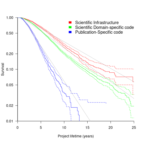
Readers familiar with academic publishing will not be surprised that projects associated with published papers have the lowest survival rate (half-life just over 2-years). Infrastructure projects are likely to be depended on by many people, who all have an interest in them surviving (half-life around 6-years). The Domain-specific half-life is around 4.5-years.
The results of this study show software systems in various research ecosystems having a range of half-lives in the same range as three major commercial software ecosystems.
Unfortunately, my experience of discussing application half-life with developers is that they believe in an imagined future where software never dies. That is, they are unwilling to consider a world where software has a high probability of being abandoned, because it requires that they consider the return on investment before spending time polishing their code.
Half-life of Microsoft products is 7 years
I get a lot of pushback from developers/managers when I tell them that the average application has a relatively short lifetime, i.e., half-life of 4-8 years. The pushback kicks in when I start citing data, up until then my listeners appear surprised/skeptical. The fact that source code has a brief and lonely existence is accepted, but telling them about the (one study) evidence that a coding mistake is more likely to disappear because of an unrelated coding change than as a result of fixing a fault report appears to make them feel uncomfortable.
Some applications live a long time, and most developers will spend most of their time working on long-lived applications. Short-lived applications are not around long enough to acquire significant developer/manager mind share.
I think the pushback is rooted in more than developer experience; developers don’t like the thought of their work disappearing from the world. The desire for permanence in what we create may be a human characteristic. Extolling the creation of reliable, maintainable, readable code creates an implicit assumption that applications are going to live long enough for the cost of these activities to be paid back.
How accurate are these half-life estimates?
The 4-8 year half-life range is derived from two datasets. A while ago I spotted another dataset: Fabiano Riccardi‘s Killed by Microsoft, currently containing information on 141 killed products.
All three datasets list just the products that have been killed, i.e., they are not a list of all products. A half-life calculation based only on killed products could underestimate the actual lifetime, it depends on whether the rate of killed products remains roughly the same percentage of all products or not. If the number of products killed, in any period, is always roughly the same percentage of all current products, then the calculated lifetime is not affected by the lack of data on the number of live products. Uncertainty in the calculated lifetime is created when the number of products killed is unconnected with the current number of live products.
It’s possible, to save money, products are more likely to be killed when a company is going through a period of poor performance, or the economy is in recession, compared to when business is booming.
Another source of uncertainty is sampling bias. Companies announce when products are released/withdrawn, creating recency bias because it’s easier to monitor the news than actively search for data on past product releases/withdraws. The plot below shows the number of products Microsoft killed in each year (red bars; post 2025 are to be killed-by dates) and number of new products launched each year blue/green line (code+data):
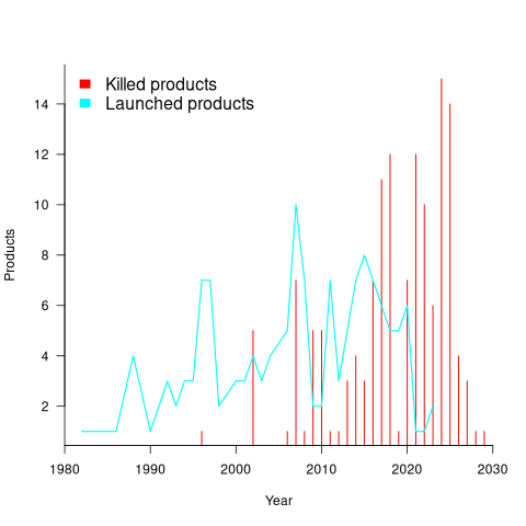
I’m sure that Microsoft killed more than one product before 2000. The Dot-com bubble burst in March 2000, and I would expect this to have resulted in lots of killed products. The lack of data on products killed before 2000 means that shorter lived products are undercounted.
The plot below shows the number of Microsoft (eventually killed) products still supported a given number of years after launch, the red line is a regression fit for products aged between 4 months and 22 years (code+data):
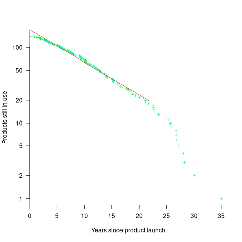
The half-life of the Microsoft products in this dataset, aged between 4 months and 22 years, is 7 years. Is the sharp decline in half-life after 22 years a real thing, or a consequence of the small amount of data before 2005? As always, more data is needed.
A distillation of Robert Glass’s lifetime experience
Robert Glass is a software engineering developer, manager, researcher and author who, until six months ago, I had vaguely heard of; somehow I had missed reading any of his 25 books. After seeing citations to some of Glass’s books, I bought half-a-dozen or so, second hand. They are well written, and twenty-five years ago I would have found them very interesting; now I simply agree with the points made.
“software creativity 2.0” is Glass’s penultimate book, published in 2006, and the one that caught my attention. I would recommend his other books to anybody who is new to software engineering, or experienced people looking for an encapsulation in print of what they encounter at work.
Glass was 74 when this book was published, having started working in computing in 1954. He was there and seems to have met many of the major names in software engineering, working with some of them.
The book is a clear-eyed summary of what Glass has learned from being involved with software engineering, and watching method/tool fashions come and go. My favourite section draws parallels between software development cultures and the culture of Rome vs. Greek vs. Barbarian:
Models Roman Greek Barbarians Organization Organize people Organize things Barely Focus Manages projects Writes programs Leap to coding Motivation Group goals Problem to be solved Heroics Working style Organizations Small groups Solo Politics Imperial Democratic Anarchist Tool use People are tools Things are tools Avoid tools Status Function-ocracy Meritocracy Fear-ocracy Activities Plan things Do things Break things Emphasize Form Substance Line of code |
The contents are essentially a collection of short essays, organized under the 19 chapter headings below, which in turn are grouped into four parts. The first nine chapters (part I, and 60% of pages) contain the experience based material, with the subsequent parts/pages having a creativity theme. A thread running through the discussion is idealism/practice:
    Discipline vs. Flexibility
    Formal methods versus Heuristics
    Optimizing versus Satisficing
    Quantitative versus Qualitative Reasoning
    Process versus Product
    Intellect vs. Clerical Tasks
    Theory vs. Practice
    Industry vs. Academe
    Fun versus Getting Serious

    Creativity in the Software Organization
    Creativity in Software Technology
    Creative Milestones in Software History

    Organizational Creativity
    The Creative Person
    Computer Support for Creativity
    Creativity Paradoxes#'twas Always Thus

    A Synergistic Conclusion
Other Conclusions |
This book deserves to be widely read. I found it best to read a single section per sitting.
The lifetime of performance coding issues
Coding activities that a developer might spend time on include: adding new functionality, fixing a reported fault, or fiddling with existing code with the intent of making it ‘better’ in some sense (which these days goes by the catch-all name of refactoring).
Improving performance, e.g., changing software to use less cpu/memory is considered, by developers, to make it ‘better’ (whether users are likely to notice the difference, or management see a ROI is for another article). There is a breed of developer whose DNA encodes for pleasure receptors that are only fire when working to reduce the amount of cpu/memory used by a program.
The paper Characterizing the evolution of statically-detectable performance issues of Android Apps by Das, Di Penta, and Malavolta studied the creation/removal of nine distinct performance coding issues in the source of 316 Android Apps (118 Apps contained five or more issues); a total of 2,408 performance issues were tracked.
What patterns might be present in the paper’s performance issues data?
I would expect there to be more creations in Apps containing more code, and more removals the longer an App is maintained; both very obvious. With more developers working on an App, there are going to be more creations and removals; do they cancel out? Management might decide to invest time in performance improvements for the next release, which would cause a spike in the number of removals per unit time.
How long do the nine performance issues survive in code, before being removed? The plot below shows the Kaplan Meier survival curve for Apps containing at least five issues (dotted blue/green are the 95% confidence intervals, code+data):
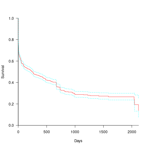
Around 15% of issues were removed on the day they are created, and by the eighth day around 30% had been removed. The roughly steady decline lasts for two-years, followed by almost stasis. Is two-years the active development lifetime of a successful Android App?
In isolation, the slope of the survival curve between eight days and two-years is not that interesting (it could be used to rule out models of the issue discovery process, e.g., happenstance discovery while working on other tasks). However, comparing it against the corresponding survival curve for reported faults tells us something about developer/management investment priorities for the two kinds of tasks, as measured by time to fix (which is a proxy for effort invested).
Unfortunately, this study did not collect information on coding mistake lifetimes, or time between a fault being reported and fixed. There have been studies investigating the survival time of coding mistakes. Reported faults should have the lowest survival rate, while the survival of coding mistakes will depend on the number of users (i.e., more users creates more opportunities to experience a fault and report it).
What factors influence performance issue time-to-fix?
The data includes information on the kind of performance issue, the number of times the App has been downloaded from the Google Play Store, and the number of contributors to the App.
Using these variables, a Cox proportional hazards model was fitted to model the survival time. In a proportional hazards model, the model coefficients are not absolute values, but provide ratio information. For instance, the following table shows the coefficients of the fitted model (code+data). Using these coefficients, we can compare the time taken to fix, say, a FloatMath issue relative to a ViewTag issue. The coefficient ratio  is the estimated ratio of fix times of the two respective issues.
Coefficient Standard error Performance issue FloatMath 0.64445 0.14175 HandlerLeak 0.69958 0.12736 Recycle 0.83041 0.11386 UseSparseArrays 0.73471 0.12493 UseValueOf 0.64263 0.11827 ViewHolder 0.87253 0.14951 ViewTag 5.24257 0.46500 Wakelock 3.34665 0.72014 Downloads 50-100 0.62490 0.26245 100-500 0.64699 0.22494 500-1000 0.56768 0.23505 1000-5000 0.50707 0.22225 5000-10000 0.53432 0.22486 10000-50000 0.62449 0.21626 50000-100000 0.42214 0.23402 100000-500000 0.21479 0.25358 1000000-5000000 0.40593 0.21851 10000000-50000000 0.03474 0.61827 100000000-500000000 0.30693 0.39868 1000000000-5000000000 0.41522 0.61599 NA 0.03868 1.02076 Contributors 1.04996 0.01265 |
There is not a lot of difference in the coefficients for the number of downloads (the model fit is poor when the Standard error is close to the Coefficient value).
The paper Investigating Types and Survivability of Performance Bugs in Mobile Apps analyses a smaller dataset of performance issue lifetimes.
Cost-effectiveness decision for fixing a known coding mistake
If a mistake is spotted in the source code of a shipping software system, is it more cost-effective to fix the mistake, or to wait for a customer to report a fault whose root cause turns out to be that particular coding mistake?
The naive answer is don’t wait for a customer fault report, based on the following simplistic argument:  .
.
where:  is the cost of fixing the mistake in the code (including testing etc), and
  is the cost of finding the mistake in the code based on a customer fault report (i.e., the sum on the right is the total cost of fixing a fault reported by a customer).
If the mistake is spotted in the code for ‘free’, then  , e.g., a developer reading the code for another reason, or flagged by a static analysis tool.
This answer is naive because it fails to take into account the possibility that the code containing the mistake is deleted/modified before any customers experience a fault caused by the mistake; let  be the likelihood that the coding mistake ceases to exist in the next unit of time.
The more often the software is used, the more likely a fault experience based on the coding mistake occurs; let  be the likelihood that a fault is reported in the next time unit.
A more realistic analysis takes into account both the likelihood of the coding mistake disappearing and a corresponding fault being reported, modifying the relationship to: *{F_{experience}/M_{gone}}")
Software systems are eventually retired from service; the likelihood that the software is maintained during the next unit of time,  , is slightly less than one.
Giving the relationship: *{F_{experience}/M_{gone}}*S_{maintained}")
which simplifies to: *{F_{experience}/M_{gone}}*S_{maintained}")
What is the likely range of values for the ratio:  ?
?
I have no find/fix cost data, although detailed total time is available, i.e., find+fix time (with time probably being a good proxy for cost). My personal experience of find often taking a lot longer than fix probably suffers from survival of memorable cases; I can think of cases where the opposite was true.
The two values in the ratio  are likely to change as a system evolves, e.g., high code turnover during early releases that slows as the system matures. The value of should decrease over time, but increase with a large influx of new users.
A study by Penta, Cerulo and Aversano investigated the lifetime of coding mistakes (detected by several tools), tracking them over three years from creation to possible removal (either fixed because of a fault report, or simply a change to the code).
Of the 2,388 coding mistakes detected in code developed over 3-years, 41 were removed as reported faults and 416 disappeared through changes to the code: 
The plot below shows the survival curve for memory related coding mistakes detected in Samba, based on reported faults (red) and all other changes to the code (blue/green, code+data):
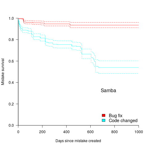
Coding mistakes are obviously being removed much more rapidly due to changes to the source, compared to customer fault reports.
For it to be cost-effective to fix coding mistakes in Samba, flagged by the tools used in this study ( is essentially one), requires:  .
.
Meeting this requirement does not look that implausible to me, but obviously data is needed.
Many coding mistakes are not immediately detectable
Earlier this week I was reading a paper discussing one aspect of the legal fallout around the UK Post-Office’s Horizon IT system, and was surprised to read the view that the Law Commission’s Evidence in Criminal Proceedings Hearsay and Related Topics were citing on the subject of computer evidence (page 204): “most computer error is either immediately detectable or results from error in the data entered into the machine”.
What? Do I need to waste any time explaining why this is nonsense? It’s obvious nonsense to anybody working in software development, but this view is being expressed in law related documents; what do lawyers know about software development.
Sometimes fallacies become accepted as fact, and a lot of effort is required to expunge them from cultural folklore. Regular readers of this blog will have seen some of my posts on long-standing fallacies in software engineering. It’s worth collecting together some primary evidence that most software mistakes are not immediately detectable.
A paper by Professor Tapper of Oxford University is cited as the source (yes, Oxford, home of mathematical orgasms in software engineering). Tapper’s job title is Reader in Law, and on page 248 he does say: “This seems quite extraordinarily lax, given that most computer error is either immediately detectable or results from error in the data entered into the machine.” So this is not a case of his words being misinterpreted or taken out of context.
Detecting many computer errors is resource intensive, both in elapsed time, manpower and compute time. The following general summary provides some of the evidence for this assertion.
Two events need to occur for a fault experience to occur when running software:
- a mistake has been made when writing the source code. Mistakes include: a misunderstanding of what the behavior should be, using an algorithm that does not have the desired behavior, or a typo,
- the program processes input values that interact with a coding mistake in a way that produces a fault experience.
That people can make different mistakes is general knowledge. It is my experience that people underestimate the variability of the range of values that are presented as inputs to a program.
A study by Nagel and Skrivan shows how variability of input values results in fault being experienced at different time, and that different people make different coding mistakes. The study had three experienced developers independently implement the same specification. Each of these three implementations was then tested, multiple times. The iteration sequence was: 1) run program until fault experienced, 2) fix fault, 3) if less than five faults experienced, goto step (1). This process was repeated 50 times, always starting with the original (uncorrected) implementation; the replications varied this, along with the number of inputs used.
How many input values needed to be processed, on average, before a particular fault is experienced? The plot below (code+data) shows the numbers of inputs processed, by one of the implementations, before individual faults were experienced, over 50 runs (sorted by number of inputs needed before the fault was experienced):
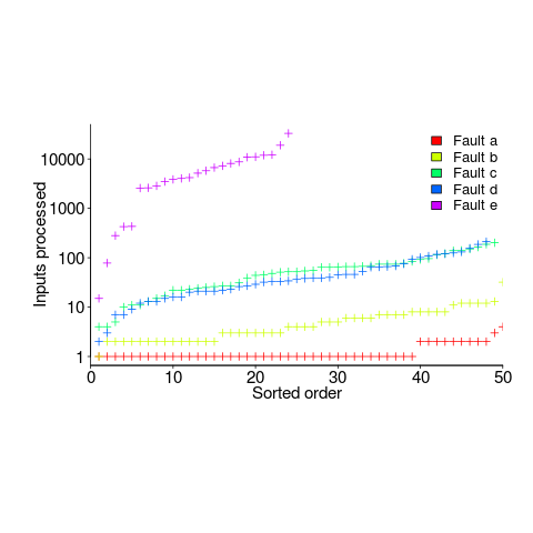
The plot illustrates that some coding mistakes are more likely to produce a fault experience than others (because they are more likely to interact with input values in a way that generates a fault experience), and it also shows how the number of inputs values processed before a particular fault is experienced varies between coding mistakes.
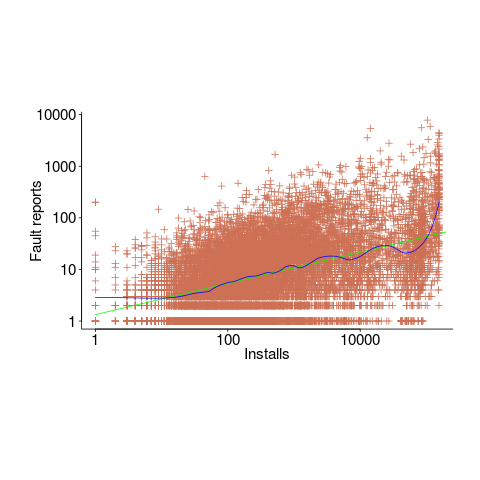
Real-world evidence of the impact of user input on reported faults is provided by the Ultimate Debian Database, which provides information on the number of reported faults and the number of installs for 14,565 packages. The plot below shows how the number of reported faults increases with the number of times a package has been installed; one interpretation is that with more installs there is a wider variety of input values (increasing the likelihood of a fault experience), another is that with more installs there is a larger pool of people available to report a fault experience. Green line is a fitted power law,  , blue line is a fitted loess model.
The source containing a mistake may be executed without a fault being experienced; reasons for this include:
- the input values don’t result in the incorrect code behaving differently from the correct code. For instance, given the made-up incorrect code
if (x < 8)(i.e.,8was typed rather than7), the comparison only produces behavior that differs from the correct code whenxhas the value7, - the input values result in the incorrect code behaving differently than the correct code, but the subsequent path through the code produces the intended external behavior.
Some of the studies that have investigated the program behavior after a mistake has deliberately been introduced include:
- checking the later behavior of a program after modifying the value of a variable in various parts of the source; the results found that some parts of a program were more susceptible to behavioral modification (i.e., runtime behavior changed) than others (i.e., runtime behavior not change),
- checking whether a program compiles and if its runtime behavior is unchanged after random changes to its source code (in this study, short programs written in 10 different languages were used),
- 80% of radiation induced bit-flips have been found to have no externally detectable effect on program behavior.
What are the economic costs and benefits of finding and fixing coding mistakes before shipping vs. waiting to fix just those faults reported by customers?
Checking that a software system exhibits the intended behavior takes time and money, and the organization involved may not be receiving any benefit from its investment until the system starts being used.
In some applications the cost of a fault experience is very high (e.g., lowering the landing gear on a commercial aircraft), and it is cost-effective to make a large investment in gaining a high degree of confidence that the software behaves as expected.
In a changing commercial world software systems can become out of date, or superseded by new products. Given the lifetime of a typical system, it is often cost-effective to ship a system expected to contain many coding mistakes, provided the mistakes are unlikely to be executed by typical customer input in a way that produces a fault experience.
Beta testing provides selected customers with an early version of a new release. The benefit to the software vendor is targeted information about remaining coding mistakes that need to be fixed to reduce customer fault experiences, and the benefit to the customer is checking compatibility of their existing work practices with the new release (also, some people enjoy being able to brag about being a beta tester).
- One study found that source containing a coding mistake was less likely to be changed due to fixing the mistake than changed for other reasons (that had the effect of causing the mistake to disappear),
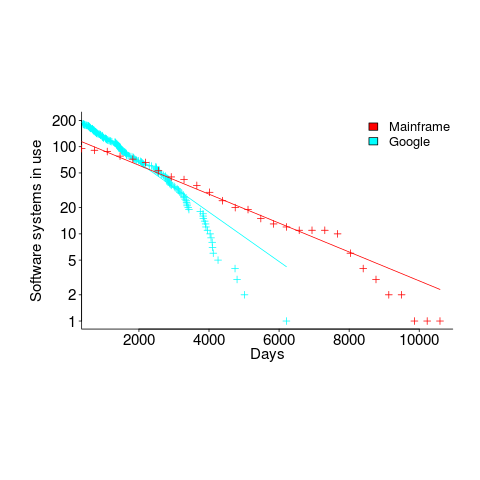
- Software systems don't live forever; systems are replaced or cease being used. The plot below shows the lifetime of 202 Google applications (half-life 2.9 years) and 95 Japanese mainframe applications from the 1990s (half-life 5 years; code+data).
Not only are most coding mistakes not immediately detectable, there may be sound economic reasons for not investing in detecting many of them.
Learning useful stuff from the Ecosystems chapter of my book
What useful, practical things might professional software developers learn from the Ecosystems chapter in my evidence-based software engineering book?
This week I checked the ecosystems chapter; what useful things did I learn (combined with everything I learned during all the other weeks spent working on this chapter)?
A casual reader would conclude that software engineering ecosystems involved lots of topics, with little or no theory connecting them. I had great plans for the connecting theories, but lack of detailed data, time and inspiration means the plans remain in my head (e.g., modelling the interaction between the growth of source code written in a particular language and the number of developers actively using that language).
For managers, the usefulness of this chapter is the strategic perspective it provides. How does what they and others are doing relate to everything else, and what patterns of evolution are to be expected?
Software people like to think that everything about software is unique. Software is unique, but the activities around it follow patterns that have been followed by other unique technologies, e.g., the automobile and jet engines. There is useful stuff to be learned from non-software ecosystems, and the chapter discusses some similarities I have learned about.
There is lots more evidence of the finite lifetime of software related items: lifetime of products, Linux distributions, packages, APIs and software careers.
Some readers might be surprised by the amount of discussion about what is now historical hardware. Software needs hardware to execute it, and the characteristics of the hardware of the day can have a significant impact on the characteristics of the software that gets written. I suspect that most of this discussion will not be that useful to most readers, but it provides some context around why things are the way they are today.
Readers with a wide knowledge of software ecosystems will notice that several major ecosystems barely get a mention. Embedded systems is a huge market, as is Microsoft Windows, and very many professional developers use C++. However, to date the focus of most research has been around Linux and Android (because its use of Java, a language often taught in academia), and languages that have a major package repository. So the ecosystems chapter presents a rather blinkered view of software engineering ecosystems.
What did I learn from this chapter?
Software ecosystems are bigger and more complicated that I had originally thought.
Readers might have a completely different learning experience from reading the ecosystems chapter. What useful things did you learn from the ecosystems chapter?
Learning useful stuff from the Projects chapter of my book
What useful, practical things might professional software developers learn from the Projects chapter in my evidence-based software engineering book?
This week I checked the projects chapter; what useful things did I learn (combined with everything I learned during all the other weeks spent working on this chapter)?
There turned out to be around three to four times more data publicly available than I had first thought. This is good, but there is a trap for the unweary. For many topics there is one data set, and that one data set may not be representative. What is needed is a selection of data from various sources, all relating to a given topic.
Some data is better than no data, provided small data sets are treated with caution.
Estimation is a popular research topic: how long will a project take and how much will it cost.
After reading all the papers I learned that existing estimation models are even more unreliable than I had thought, and what is more, there are plenty of published benchmarks showing how unreliable the models really are (these papers never seem to get cited).
Models that include lines of code in the estimation process (i.e., the majority of models) need a good estimate of the likely number of lines in the final software system. One issue that nobody had considered was the impact of developer variability on the number of lines written to implement the same functionality, which turns out to be large. Oops.
Machine learning has infested effort estimation research. What the machine learning models actually do is estimate adjustment, i.e., they do not create their own estimate but adjust one passed in as input to the model. Most estimation data sets are tiny, and only contain a few different variables; unless the estimate is included in the training phase, the generated model produces laughable results. Oops.
The good news is that there appear to be lots of recurring patterns in the project data. This is good news because recurring patterns are something to be explained by a theory of software project development (apparent randomness is bad news, from the perspective of coming up with a model of what is going on). I think we are still a long way from having workable theories, but seeing patterns is a good sign that one or more theories will be possible.
I think that the main takeaway from this chapter is that software often has a short lifetime. People in industry probably have a vague feeling that this is true, from experience with short-lived projects. It is not cost effective to approach commercial software development from the perspective that the code will live a long time; some code does live a long time, but most dies young. I see the implications of this reality being a major source of contention with those in academia who have spent too long babbling away in front of teenagers (teaching the creation of idealized software that lives on forever), and little or no time building software systems.
A lot of software is written by teams of people, however, there is not a lot of data available on teams (software or otherwise). Given the difficulty of hiring developers, companies have to make do with what they have, so a theory of software teams might not be that useful in practice.
Readers might have a completely different learning experience from reading the projects chapter. What useful things did you learn from the projects chapter?
Recent Comments