Archive
Criteria for increased productivity investment
You have a resource of  person days to implement a project, and believe it is worth investing some of these days,
  , to improve team productivity (perhaps with training, or tooling). What is the optimal amount of resource to allocate to maximise the total project work performed (i.e., excluding the performance productivity work)?
Without any productivity improvement, the total amount of project work is:
") , where
, where ") is the starting team productivity function, f, i.e., with zero investment.
is the starting team productivity function, f, i.e., with zero investment.
After investing person days to increase team productivity, the total amount of project work is now:
*f(I)") , where
, where ") is the team productivity function, f, after the investment .
is the team productivity function, f, after the investment .
To find the value of that maximises  , we differentiate with respect to , and solve for the result being zero:
*f prime(I)-f(I) =0") , where
, where ") is the differential of the yet to be selected function
is the differential of the yet to be selected function  .
.
Rearranging this equation, we get:
}/{D*f prime(I)}")
We can plug in various productivity functions, , to find the optimal value of .
For a linear relationship, i.e., =p*I*f(0)") , where
, where  is the unit productivity improvement constant for a particular kind of training/tool, the above expression becomes:

Rearranging, we get:  , or
, or  .
.
The surprising (at least to me) result that the optimal investment is half the available days.
It is only worthwhile making this investment if it increases the total amount of project work. That is, we require:  < (D-I)*f(I)") .
.
For the linear improvement case, this requirement becomes:
*p*{D/2}") , or
, or 
This is the optimal case, but what if the only improvement options available are not able to sustain a linear improvement rate of at least  ? How many days should be invested in this situation?
A smaller investment,  , is only worthwhile when:
 < (D-s)*f(s)") , where
, where  , and
, and  .
.
Substituting gives:  < (D-k*D)*r*k*D*f(0)") , which simplifies to:
, which simplifies to:
} < r")
The blue/green line plot below shows the minimum value of  for
for  (and
(and  , increasing moves the line down), with the red line showing the optimal value
  . The optimal value of
  is at the point where has its minimum worthwhile value (the derivative of
 }") is
is ^2}") ; code):
; code):
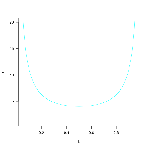
This shows that it is never worthwhile making an investment when:  , and that when it is always worthwhile investing , with any other value either wasting time or not extracting all the available benefits.
In practice, an investment may be subject to diminishing returns.
When the rate of improvement increases as the square-root of the number of days invested, i.e., =p*sqrt{I}*f(0)") , the optimal investment, and requirement on unit rate are as follows:
, the optimal investment, and requirement on unit rate are as follows:
only invest:  , when:
If the rate of improvement with investment has the form:  , the respective equations are:
only invest:  , when:
 ^{q+1}/{q^q D^q} < r") . The minimal worthwhile value of always occurs at the optimal investment amount.
. The minimal worthwhile value of always occurs at the optimal investment amount.
When the rate of improvement is logarithmic in the number of days invested, i.e., =p*log{I}*f(0)") , the optimal investment, and requirement on unit rate are as follows:
, the optimal investment, and requirement on unit rate are as follows:
only invest: -1}") , where
, where  is the Lambert W function, when:
 -1})(W(e*D)-1)} < r")
These expressions can be simplified using the approximation  approx log(x)-log(log(x))") , giving:
, giving:
only invest: }") , when:
, when: }/{(2+log(D))(log(D)-log(1+log(D)))} < r")
In practice, after improving rapidly, further investment on improving productivity often produces minor gains, i.e., the productivity rate plateaus. This pattern of rate change is often modelled using a logistic equation, e.g.,  .
.
However, following the process used above for this logistic equation produces an equation for , -1}/c") , that does not have any solutions when
, that does not have any solutions when  and are positive.
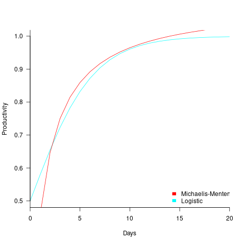
The problem is that the derivative goes to zero too quickly. The Michaelis-Menten equation,  , has an asymptotic limit whose derivative goes to zero sufficiently slowly that a solution is available.
only invest:  , when
The plot below shows example Michaelis-Menten and Logistic equations whose coefficients have been chosen to produce similar plots over the range displayed (code):
These equations are all well and good. The very tough problem of estimating the value of the coefficients is left to the reader.
This question has probably been answered before. But I have not seen it written down anywhere. References welcome.
Break even ratios for development investment decisions
Developers are constantly being told that it is worth making the effort when writing code to make it maintainable (whatever that might be). Looking at this effort as an investment what kind of return has to be achieved to make it worthwhile?
Short answer: The percentage saving during maintenance has to be twice as great as the percentage investment during development to break even, higher ratio to do better.
The longer answer is below as another draft section from my book Empirical software engineering with R book. As always comments and pointers to more data welcome. R code and data here.
Break even ratios for development investment decisions
Upfront investments are often made during software development with the aim of achieving benefits later (e.g., reduced cost or time). Examples of such investments include spending time planning, designing or commenting the code. The following analysis calculates the benefit that must be achieved by an investment for that investment to break even.
While the analysis uses years as the unit of time it is not unit specific and with suitable scaling months, weeks, hours, etc can be used. Also the unit of development is taken to be a complete software system, but could equally well be a subsystem or even a function written by one person.
Let  be the original development cost and
  the yearly maintenance costs, we start by keeping things simple and assume is the same for every year of maintenance; the total cost of the system over
  years is:

If we make an investment of  % in reducing future maintenance costs with the expectations of achieving a benefit of
  %, the total cost becomes:
 + y*m*(1+i)*(1-b)")
and for the investment to break even the following inequality must hold:
 + y*m*(1+i)*(1-b) < d + y*m")
expanding and simplifying we get:

or:

If the inequality is true the ratio  is the primary contributor to the right-hand-side and must be greater than 1.
A significant problem with the above analysis is that it does not take into account a major cost factor; many systems are replaced after a surprisingly short period of time. What relationship does the ratio need to have when system survival rate is taken into account?
Let be the percentage of systems that survive each year, total system cost is now:

where *(1-b)")
Summing the power series for the maximum of years that any system in a company’s software portfolio survives gives:
}/{1 - s}")
and the break even inequality becomes:
} < {b}/{i} + b")
The development/maintenance ratio is now based on the yearly cost multiplied by a factor that depends on the system survival rate, not the total maintenance cost
If we take >= 5 and a survival rate of less than 60% the inequality simplifies to very close to:

telling us that if the yearly maintenance cost is equal to the development cost (a situation more akin to continuous development than maintenance and seen in 5% of systems in the IBM dataset below) then savings need to be at least twice as great as the investment for that investment to break even. Taking the mean of the IBM dataset and assuming maintenance costs spread equally over the 5 years, a break even investment requires savings to be six times greater than the investment (for a 60% survival rate).
The plot below gives the minimum required saving/investment ratio that must be achieved for various system survival rates (black 0.9, red 0.8, blue 0.7 and green 0.6) and development/yearly maintenance cost ratios; the line bundles are for system lifetimes of 5.5, 6, 6.5, 7 and 7.5 years (ordered top to bottom)
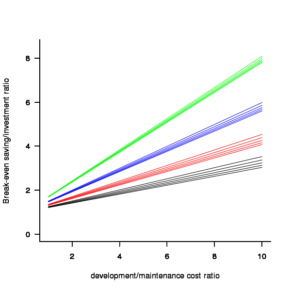
Figure 1. Break even saving/investment ratio for various system survival rates (black 0.9, red 0.8, blue 0.7 and green 0.6) and development/maintenance ratios; system lifetimes are 5.5, 6, 6.5, 7 and 7.5 years (ordered top to bottom)
Development and maintenance costs
Dunn’s PhD thesis <book Dunn_11> lists development and total maintenance costs (for the first five years) of 158 software systems from IBM. The systems varied in size from 34 to 44,070 man hours of development effort and from 21 to 78,121 man hours of maintenance.
The plot below shows the ratio of development to five year maintenance costs for the 158 software systems. The mean value is around one and if we assume equal spending during the maintenance period then  .
.
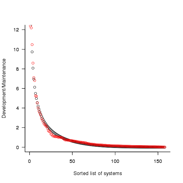
Figure 2. Ratio of development to five year maintenance costs for 158 IBM software systems sorted in size order. Data from Dunn <book Dunn_11>.
The best fitting common distribution for the maintenance/development ratio is the <Beta distribution>, a distribution often encountered in project planning.
Is there a correlation between development man hours and the maintenance/development ratio (e.g., do smaller systems tend to have a lower/higher ratio)? A Spearman rank correlation test between the maintenance/development ratio and development man hours gives:
|
showing very little connection between the two values.
Is the data believable?
While a single company dataset might be thought to be internally consistent in its measurement process, IBM is a very large company and it is possible that the measurement processes used were different.
The maintenance data applies to software systems that have not yet reached the end of their lifespan and is not broken down by year. Any estimate of total or yearly maintenance can only be based on assumptions or lifespan data from other studies.
System lifetime
A study by Tamai and Torimitsu <book Tamai_92> obtained data on the lifespan of 95 software systems. The plot below shows the number of systems surviving for at least a given number of years and a fit of an <Exponential distribution> to the data.
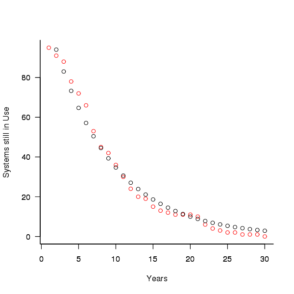
Figure 3. Number of software systems surviving to a given number of years (red) and an exponential fit (black, data from Tamai <book Tamai_92>).
The nls function gives  as the best fit, giving a half-life of 5.4 years (time for the number of systems to reduce by 50%), while rounding to
  gives a half-life of 6.6 years and reducing to
  a half life of 4.6 years.
It is worrying that such a small change to the estimated fit can have such a dramatic impact on estimated half-life, especially given the uncertainty in the applicability of the 20 year old data to today’s environment. However, the saving/investment ratio plot above shows that the final calculated value is not overly sensitive to number of years.
Is the data believable?
The data came from a questionnaire sent to the information systems division of corporations using mainframes in Japan during 1991.
It could be argued that things have stabilised over the last 20 years ago and complete software replacements are rare with most being updated over longer periods, or that growing customer demands is driving more frequent complete system replacement.
It could be argued that large companies have larger budgets than smaller companies and so have the ability to change more quickly, or that larger companies are intrinsically slower to change than smaller companies.
Given the age of the data and the application environment it came from a reasonably wide margin of uncertainty must be assigned to any usage patterns extracted.
Summary
Based on the available data an investment during development must recoup a benefit during maintenance that is at least twice as great in percentage terms to break even:
- systems with a yearly survival rate of less than 90% must have a benefit/investment rate greater than two if they are to break even,
- systems with a development/yearly maintenance rate of greater than 20% must have a benefit/investment rate greater than two if they are to break even.
The availanble software system replacement data is not reliable enough to suggest any more than that the estimated half-life might be between 4 and 8 years.
This analysis only considers systems that have been delivered and started to be used. Projects are cancelled before reaching this stage and including these in the analysis would increase the benefit/investment break even ratio.
Recent Comments