Archive
Extracting numbers from a stacked density plot
A month or so ago, I found a graph showing a percentage of PCs having a given range of memory installed, between March 2000 and April 2020, on a TechTalk page of PC Matic; it had the form of a stacked density plot. This kind of installed memory data is rare, how could I get the underlying values (a previous post covers extracting data from a heatmap)?
The plot below is the image on PC Matic’s site:
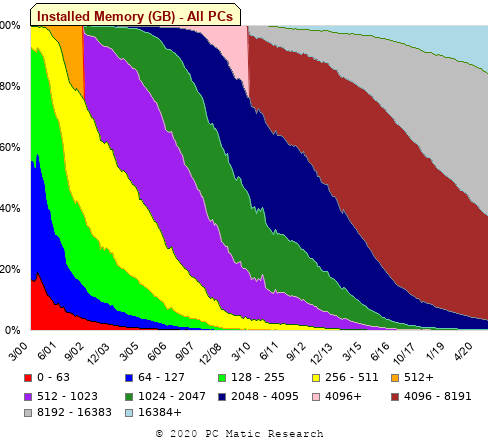
The change of colors creates a distinct boundary between different memory capacity ranges, and it ought to be possible to find the y-axis location of each color change, for a given x-axis location (with location measured in pixels).
The image was a png file, I loaded R’s png package, and a call to readPNG created the required 2-D array of pixel information.
library("png")
img=readPNG("../rc_mem_memrange_all.png") |
Next, the horizontal and vertical pixel boundaries of the colored data needed to be found. The rectangle of data is surrounded by white pixels. The number of white pixels (actually all ones corresponding to the RGB values) along each horizontal and vertical line dramatically drops at the data image boundary. The following code counts the number of col points in each horizontal line (used to find the y-axis bounds):
horizontal_line=function(a_img, col)
{
lines_col=sapply(1:n_lines, function(X) sum((a_img[X, , 1]==col[1]) &
                                            (a_img[X, , 2]==col[2]) &
                                            (a_img[X, , 3]==col[3]))
                )

return(lines_col)
}

white=c(1, 1, 1)
n_cols=dim(img)[2]

# Find where fraction of white points on a line changes dramatically
white_horiz=horizontal_line(img, white)

# handle when upper boundary is missing
ylim=c(0, which(abs(diff(white_horiz/n_cols)) > 0.5))
ylim=ylim[2:3] |
Next, for each vertical column of pixels, at each x-axis pixel location, the sought after y value occurs at the change of color boundary in the corresponding vertical column. This boundary includes a 1-pixel wide separation color, which creates a run of 2 or 3 consecutive pixel color changes.
The color change is easily found using the duplicated function.
# Return y position of vertical color changes at x_pos
y_col_change=function(x_pos)
{
# Good enough technique to generate a unique value per RGB color
col_change=which(!duplicated(img[y_range, x_pos, 1]+
                          10*img[y_range, x_pos, 2]+
                         100*img[y_range, x_pos, 3]))

# Handle a 1-pixel separation line between colors.
# Diff is used to find these consecutive sequences.
y_change=c(1, col_change[which(diff(col_change) > 1)+1])

# Always return a vector containing max_vals elements.
return(c(y_change, rep(NA, max_vals-length(y_change))))
} |
Next, we need to group together the sequence of points that delimit a particular boundary. The points along the same boundary are all associated with the same two colors, i.e., the ones below/above the boundary (plus a possible boundary color).
The plot below shows all the detected boundary points, in black, overwritten by colors denoting the points associated with the same below/above colors (code):
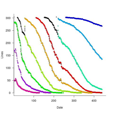
The visible black pluses show that the algorithm is not perfect. The few points here and there can be ignored, but the two blocks at the top of the original image have thrown a spanner in the works for some range of points (this could be fixed manually, or perhaps it is possible to tweak the color extraction formula to work around them).
How well does this approach work with other stacked density plots? No idea, but I am on the lookout for other interesting examples.
A first stab a low resolution image enhancement
Team Clarify-the-Heat (Gary, Pavel and yours truly) were at a hackathon sponsored by Flir at the weekend.
The FlirONE contains an infrared sensor with 160 by 120 pixels, plus an optical sensor that provides a higher resolution image that can be overlaid with the thermal, that attaches to the USB port of an Android phone or iPhone. The sensor frequency range is 8 to 14 µm, i.e., ‘real’ infrared, not the side-band sliver obtained by removing the filter from visual light sensors.
At 160 by 120 the IR sensor resolution is relatively low, compared to today’s optical sensors, and team Clarify-the-Heat decided to create an iPhone App that merged multiple images to create a higher resolution image (subpixel interpolation) in real-time. An iPhone was used because the Flir software for this platform has been around longer (Android support is on its first release) and image processing requires lots of cpu power (i.e., compiled Objective-C is likely to be a lot faster than interpreted Java). The FlirONE frame rate is 8.6 images per second.
Modern smart phones contain 3-axis gyroscopes and data on change of rotational orientation was used to find the pixels from two images that corresponded to the same area of the viewed 2-D image. Phone gyroscope sensors drift over periods of a few seconds, some experimentation found that over a period of a few seconds the drift on Gary’s iPhone was safely under a tenth of a degree; one infrared pixel had a field of view of approximately 1/3 degrees horizontally and 1/4 degrees vertically. Some phone gyroscope sensors are known to be sensitive enough to pick up the vibrations caused by local conversations.
The plan was to get an App running in realtime on the iPhone. In practice debugging a couple of problems ate up the hours and the system demonstrated uploaded data from the iPhone to a server which a laptop read and processed two images to create a higher resolution result (the intensity from the overlapping pixels is averaged to double, in our case, the resolution). This approach is very primitive compared to the algorithms that do sub-pixel enhancement by detecting image features (late in the day we found out that OpenCV supports some of this kind of stuff), but it requires image less image processing and should be practical in real-time on a phone.
We discovered that the ‘raw’ data returned by the FlirONE API has been upsampled to produce a 320 by 240 image. This means that the gyroscope data, used to align image pixels, has to be twice as accurate. We did not try to use magnetic field data (while not accurate the values do not drift) to filter the gyroscope readings.
Two IR images from a FlirOne, of yours truly, and a ‘higher’ resolution image below:
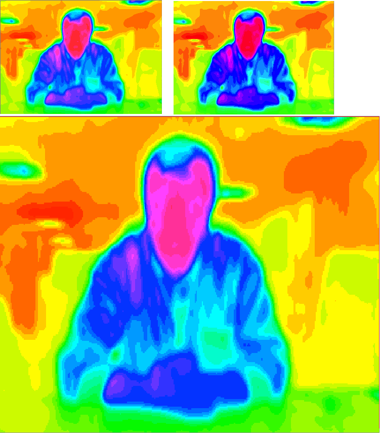
The enhanced image shows more detail in places, but would obviously benefit from input from more images. The technique relies on partial overlap between pixels, which is a hit and miss affair (we were managing to extract around 5 images per second but did not get as far as merging more than two images at a time).
Team Clarify-the_Heat got an honorable mention, but then so did half the 13 teams present, and I won a FlirONE in one of the hourly draws 🙂 It looks like they will be priced around $250 when they go on sale in mid-August. I wonder how long it will take before they are integrated into phones (yet more megapixels in the visual spectrum is a bit pointless)?
I thought the best project of the event was by James Rampersad, who used processed the IR video stream using Eulerian Video Magnification to how blood pulsing through his face.
Recent Comments