Archive
COCOMO: Not worth serious attention
The Constructive Cost Model (COCOMO) was introduced to the world by the book “Software Engineering Economics” by Barry Boehm; this particular version of the model is now known by the year of publication, COCOMO 81. The book describes a model that estimates software project cost drivers, such as effort (in man months) and elapsed time; the data from the 63 projects used to help calibrate the equations appears on pages 496-497.
Only having 63 measurements to model such a complex problem means any predictions will have very wide error bounds; however, the small amount of data did not stop Boehm building an academic career out of over-fitting these 63 measurements using 17 input parameters (the COCOMO II book came out in 2000 and was initially calibrated by fitting 22 parameters to 83 measurement points and then by fitting 23 parameters to 161 measurement points; the measurement data does not appear to be publicly available).
A sentence on page 493 suggests that over-fitting may not be the only problem to be found in the data analysis: “The calibration and evaluation of COCOMO has not relied heavily on advanced statistical techniques.”
Let’s take the original data and duplicate the original analysis, before trying something more advanced (code+data).
A central plank of the COCOMO model is the equation:  , where
  is total effort in man months,
  a constant obtained by fitting the data,
  thousands of lines of source code and
  a constant obtained by fitting the data.
This post discusses fitting this equation for the three modes of software projects defined by Boehm (along with the equations he fitted):
- Organic, relatively small teams operating in a highly familiar environment:
 ,
, - Embedded, the product has to operate within strongly coupled, complex, hardware, software and operational procedures such as air traffic control:
 ,
, - Semidetached, an intermediate stage between the two extremes:
 .
.
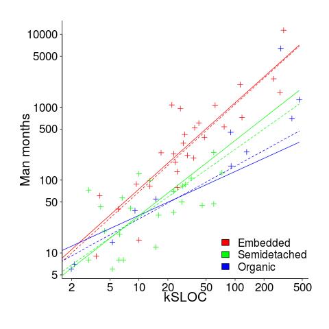
The plot below shows kSLOC against Effort, with solid lines fitted using what I guess was Boehm’s approach and dashed lines showing fitted lines after removing outliers (Figure 6-5 in the book has the x/y axis switched; the points in the above plot appear to match those in this figure):
The fitted equations are (the standard error on the multiplier, , is around ±30%, while on the exponent, , the absolute value varies between ±0.1 and ±0.2):
- Organic:
 , after outlier removal
- Embedded:
 , after outlier removal
- Semidetached:
 , after outlier removal
  .
.
The only big difference is for Organic, which is very different. My first reaction on seeing this was to double check the values used against those in the book. How did Boehm make such a big mistake and why has nobody spotted it (or at least said anything) before now? Papers by Boehm’s students do use fancy statistical techniques and contain lots of tables of numbers relating to COCOMO 81, but no mention of what model they actually found to be a good fit.
The table on pages 496-497 contains man month estimates made using Boehm’s equations (the EST column). The values listed are a close match to the values I calculated using Boehm’s Semidetached equation, but there are many large discrepancies between printed values and values I calculated (using Boehm’s equations) for Organic and Embedded. If the data in this table contains a lot of mistakes, it may explain why I get very different values fitting the data for Organic. Some ther columns contain values calculated using the listed EST values and the few I have checked are correct, so if there was an error in the EST value calculation it must have occurred early in the chain of calculations.
The data for each of the three modes of software development contain several in your face outliers (assuming the values are correct). Based on the fitted equations is does not look like Boehm removed these (perhaps detecting outliers is an advanced technique).
Once the very obvious outliers are removed the quadratic equation,  , becomes a viable competing model. Unfortunately we don’t have enough data to do a serious comparison of this equation against the COCOMO equation.
In practice the COCOMO 81 model has been found to be highly inaccurate and very much dependent upon the interpretation of the input parameters.
Further down on page 493 we have: “I have become convinced that the software field is currently too primitive, and cost driver interaction too complex, for standard statistical techniques to make much headway;”.
With so much complexity and uncertainty, careful application of statistical techniques is the only way of reliable way of distinguishing any signal from noise.
COCOMO does not deserve anymore serious attention (the code+data includes some attempts to build alternative models, before I decided it was not worth the effort).
Recent Comments