Archive
Advertised prices of desktop computers during the 1990s
The 1990s was a decade of dramatic improvements in desktop computer capacity and performance. The difference in performance between the newest and current systems was clearly visible from the rate at which compiler messages zipped up the screen. How did the price of these desktop systems change during this period?
Magazine adverts are sometimes the only publicly available source of information about historical products. For instance, the characteristics of IBM PC compatible computers (e.g., price, RAM, clock frequency) over the first 20 years since they were first introduced in the early 1980s.
During the 1980s and 1990s BYTE magazine was the leading monthly computer magazine in the US, with a strong following here in the UK. Each issue contained around 400+ pages, and was packed with adverts from all the major hardware/software vendors. The last issue appeared in Jul 1998. The Internet Archive contains a scanned copy of every issue.
In 1987 Dell Computer Corp started selling cut-price computers direct to customers. Dell ran adverts in every issue of BYTE from June 1988 until the magazine closed. Gateway was another company in this market, and also regularly advertised in BYTE.
The text information present in adverts is often embedded within graphical content. My interest in this information has not been sufficient to manually type it in. LLMs are now available, and these have proven to be remarkably effective at extracting information from images.
The following advert shows how information specific to a particular computer system appears once, along with prices for particular options. Grok correctly populates a csv file containing information on four systems.
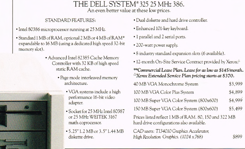
I did not attempt to ask LLMs to extract the Dell/Gateway ads from a 400+ page magazine. Manual extraction of the advert pages also gave me the opportunity to scan for other ads (a few companies advertised sporadically, e.g., Micron). Some experimentation showed that Grok returned the most accurate/reliable data.
System configuration information, for Dell and Gateway, was extracted from their adverts that appeared in the June/December issues for every year between 1988 and 1998.
Adverts show the price of particular system configurations. Typically, vendors list prices for minimal systems, along with the incremental price for more memory or a larger hard disc.
The plot below shows the original US dollar prices of 500 systems appearing in Dell/Gateway/Micron/Zeos BYTE adverts during the 1990s (code+data):
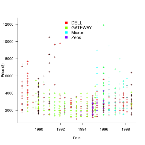
These prices have not been adjusted for inflation, and show the numeric values often ending in “99” that appeared in the adverts.
Once a ballpark figure is established in the market for the price of a product, vendors are loath to decrease it. Higher priced systems generally have higher profit margins.
Dell starts by offering systems whose price varies by a factor of four, and then settles into a narrower range of prices (presumably based on feedback from volume of sales). Micro appears to be similarly experimenting around 1996.
In the UK, when the price of low-end systems reached £1,000, rather than continuing to reduce the price, sales outlets started adding a printer to a complete package, keeping the price at around £1,000 (which families were willing to pay). Eventually the cost of a printer was not enough to fill the price gap.
The plot below shows the advertised disk size and amount of RAM installed in 500 systems advertised during the 1990s (the 1.44MB disk is a floppy drive only system; code+data):
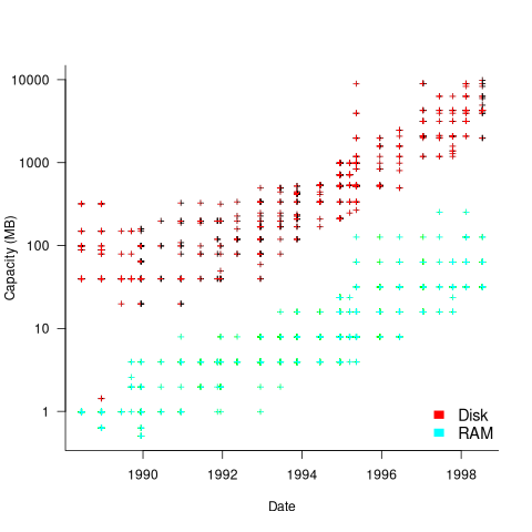
The well-known exponential capacity growth is clearly visible.
The data shows that during the 1990 there was no consistent decrease in the numeric value of the advertised price of desktop computers, which fluctuated (more data is needed to separate out the effects of functionality added to top-end systems), while actual prices decreased by 30% over the decade due to inflation. The capacity of the disk and RAM installed in desktop systems increased exponentially (also cpu clock speed; this plot is not shown).
The Hedonic index is a process used by economists to model the interaction of a product’s price and its characteristics.
The 2024 update to my desktop system
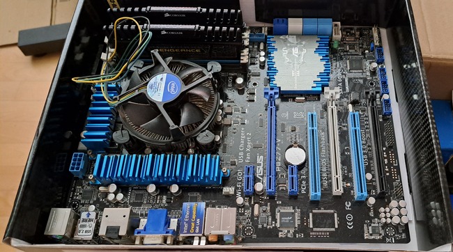
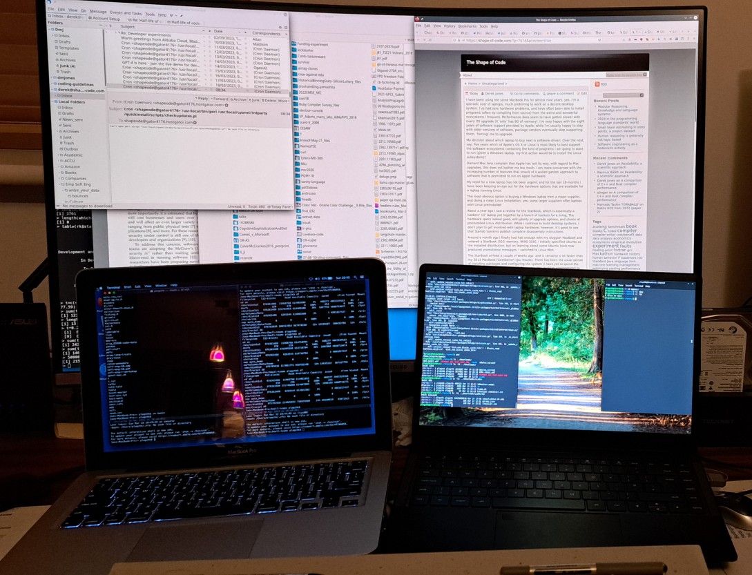
I have just upgraded my desktop system. As you can see from the picture below, it is a bespoke system; the third system built using the same chassis.
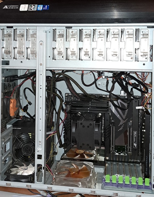
The 11 drive bays on the right are configured for six 5.25-inch and five 3.5-inch disks/CD/DVD/tape drives, there is a drive cage that fits above the power supply (top left) that holds another three 3.5-inch devices. The central black rectangle with two sets of four semicircular caps (fan above/below) is the cpu cooling tower, with two 32G memory sticks immediately to its right. The central left fan is reflected in a polished heatsink.
Why so many bays for disks?
The original need, in 2005 (well before GitHub), was for enough storage to hold the source code available, via ftp, from various hosting sites that were springing up, hence the choice of the Thermaltake Armour Series VA8000BWS Supertower. The first system I built contained six 400G Barracuda drives
The original power supply, a Thermaltake Silent Purepower 680W PSU, with its umpteen power connectors is still giving sterling service (black box with black fan at top left).
When building a system, I start by deciding on the motherboard. Boards supporting 6+ SATA connectors were once rare, but these days are more common on high-end systems. I also look for support for the latest cpu families and high memory bandwidth. I’m not a gamer, so no interest in graphics cards.
The three systems are:
- in 2005, an ASUS A8N-SLi Premium Socket 939 Motherboard, an AMD Athlon 64 X2 Dual-Core 4400 2.2Ghz cpu, and Corsair TWINX2048-3200C2 TwinX (2 x 1GB) memory. A Red Hat Linux distribution was installed,
- in 2013, an intermittent problem appeared on the A8N motherboard, so I upgraded to an ASUS P8Z77-V 1155 Socket motherboard, an Intel Core i5 Ivy Bridge 3570K – 3.4 GHz cpu, and Corsair CMZ16GX3M2A1600C10 Vengeance 16GB (2x8GB) DDR3 1600 MHz memory. Terabyte 3.25-inch disk drives were now available, and I installed two 2T drives. A openSUSE Linux distribution was installed.
The picture below shows the P8Z77-V, with cpu+fan and memory installed, sitting in its original box. This board and the one pictured above are the same length/width, i.e., the ATX form factor. This board is a lot lighter, in color and weight, than the Z790 board because it is not covered by surprisingly thick black metal plates, intended to spread areas of heat concentration,
- in 2024, there is no immediate need for an update, but the 11-year-old P8Z77 is likely to become unreliable sooner rather than later, better to update at a time of my choosing. At £400 the ASUS ROG Maximus Z790 Hero LGA 1700 socket motherboard is a big step up from my previous choices, but I’m starting to get involved with larger datasets and running LLMs locally. The Intel Core i7-13700K was chosen because of its 16 cores (I went for a hefty cooler upHere CPU Air Cooler with two fans), along with Corsair Vengeance DDR5 RAM 64GB (2x32GB) 6400 memory. A 4T and 8T hard disk, plus a 2T SSD were added to the storage system. The Linux Mint distribution was installed.
The last 20-years has seen an evolution of the desktop computer I own: roughly a factor of 10 increase in cpu cores, memory and storage. Several revolutions occurred between the roughly 20 years from the first computer I owned (an 8-bit cpu running at 4 MHz with 64K of memory and two 360K floppy drives) and the first one of these desktop systems.
What might happen in the next 20-years?
Will it still be commercially viable for companies to sell motherboards? If enough people switch to using datacenters, rather than desktop systems, many companies will stop selling into the computer component market.
LLMs perform simple operations on huge amounts of data. The bottleneck is transferring the data from memory to the processors. A system where simple compute occurs within the memory system would be a revolution in mainstream computer architecture.
Motherboards include a socket to support a specialised AI chip, like the empty socket for Intel’s 8087 on the original PC motherboards, is a reuse of past practices.
Relative performance of computers from the 1950s/60s/70s
What was the range of performance of computers introduced in the 1950, 1960s and 1970s, and what was the annual rate of increase?
People have been measuring computer performance since they were first created, and thanks to the Internet Archive the published results are sometimes available today. The catch is that performance was often measured using different benchmarks. Fortunately, a few benchmarks were run on many systems, and in a few cases different benchmarks were run on the same system.
I have found published data on four distinct system performance estimation models, with each applied to 100+ systems (a total of 1,306 systems, of which 1,111 are unique). There is around a 20% overlap between systems across pairs of models, i.e., multiple models applied to the same system. The plot below shows the reported performance for pairs of estimates for the same system (code+data):

The relative performance relationship between pairs of different estimation models for the same system is linear (on a log scale).
Each of the models aims to produce a result that is representative of typical programs, i.e., be of use to people trying to decide which system to buy.
- Kenneth Knight built a structural model, based on 30 or so system characteristics, such as time to perform various arithmetic operations and I/O time; plugging in the values for a system produced a performance estimate. These characteristics were weighted based on measurements of scientific and commercial applications, to calculate a value that was representative of scientific or commercial operation. The Knight data appears in two magazine articles analysing systems from the 1950s and 1960s (the 310 rows are discussed in an earlier post), and the 1985 paper “A functional and structural measurement of technology”, containing data from the late 1960s and 1970s (120 rows),
- Ein-Dor and Feldmesser also built a structural model, based on the characteristics of 209 systems introduced between 1981 and 1984,
- The November 1980 Datamation article by Edward Lias lists what he called the KOPS (thousands of operations per second, i.e., MIPS for slower systems) value for 237 systems. Similar to the Knight and Ein-dor data, the calculated value is based on weighting various cpu instruction timings
- The Whetstone benchmark is based on running a particular program on a system, and recording its performance; this benchmark was designed to be representative of scientific and engineering applications, i.e., floating-point intensive. The design of this benchmark was the subject of last week’s post. I extracted 504 results from Roy Longbottom’s extensive collection of Whetstone results going back to the mid-1960s.
While the Whetstone benchmark was originally designed as an Algol 60 program that was representative of scientific applications written in Algol, only 5% of the results used this version of the benchmark; 85% of the results used the Fortran version. Fitting a regression model to the data finds that the Fortran version produced higher results than the Algol 60 version (which would encourage vendors to use the Fortran version). To ensure consistency of the Whetstone results, only those using the Fortran benchmark are used in this analysis.
A fifth dataset is the Dhrystone benchmark followed in the footsteps of the Whetstone benchmark, but targetting integer-based applications, i.e., no floating-point. First published in 1984, most of the Dhrystone results apply to more recent systems than the other benchmarks. This code+data contains the 328 results listed by the Performance Database Server.
Sometimes slightly different system names appear in the published results. I used the system names appearing in the Computers Models Database as the definitive names. It is possible that a few misspelled system names remain in the data (the possible impact is not matching systems up across models), please let me know if you spot any.
What is the best statistical technique to use to aggregate results from multiple models into a single relative performance value?
I came up with various possibilities, none of which looked that good, and even posted a question on Cross Validated (no replies yet).
Asking on the Evidence-based software engineering Discord channel produced a helpful reply from Neal Fultz, i.e., use the random effects model: lmer(log(metric) ~ (1|System)+(1|Bench), data=Sall_clean) ; after trying lots of other more complicated approaches, I would probably have eventually gotten around to using this approach.
Does this random effects model produce reliable values?
I don’t have a good idea how to evaluate the fitted model. Looking at pairs of systems where I know which is faster, the relative model values are consistent with what I know.
A csv of the calculated system relative performance values. I have yet to find a reliable way of estimating confidence bounds on these values.
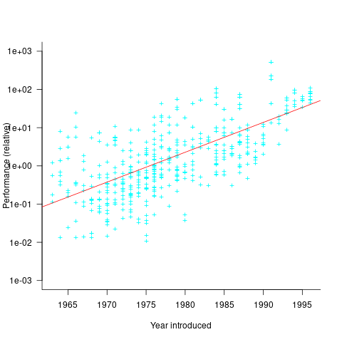
The plot below shows the performance of systems introduced in a given year, on a relative scale, red line is a fitted exponential model (a factor of 5.5 faster, annually; code+data):
If you know of a more effective way of analysing this data, or any other published data on system benchmarks for these decades, please let me know.
Hardware/Software cost ratio folklore
What percentage of data processing budgets is spent on software, compared to hardware?
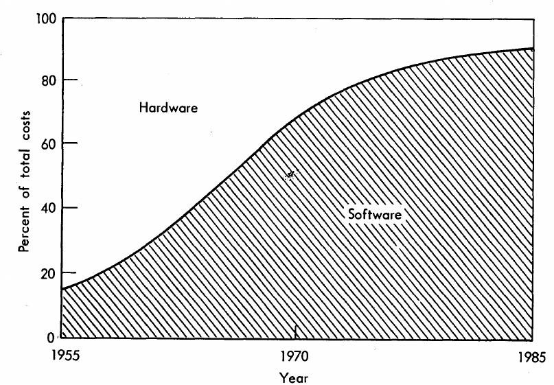
The information in the plot below quickly became, and remains, the accepted wisdom, after it was published in May 1973 (page 49).
Is this another tale from software folklore? What does the evidence have to say?
What data did Barry Boehm use as the basis for this 1973 article?
Volume IV of the report Information processing/data automation implications of Air-Force command and control requirements in the 1980s (CCIP-85)(U), Technology trends: Software, contains this exact same plot, and Boehm is a co-author of volume XI of this CCIP-85 report (May 1972).
Neither the article or report explicitly calls out specific instances of hardware/software costs. However, Boehm’s RAND report Software and Its Impact A Quantitative Assessment (Dec 1972) gives three examples: the US Air Force estimated they will spend three times as much on software compared to hardware (in early 1970s), a military C&C system ($50-100 million hardware, $722 million software), and recent NASA expenditure ($100 million hardware, $200 million software; page 41).
The 10% hardware/90% software division by 1985 is a prediction made by Boehm (probably with others involved in the CCIP-85 work).
What is the source for the 1955 percentage breakdown? The 1968 article Software for Terminal-oriented systems (page 30) by Werner L. Frank may provide the answer (it also makes a prediction about future hardware/software cost ratios). The plot below shows both the Frank and Boehm data based on values extracted using WebPlotDigitizer (code+data):
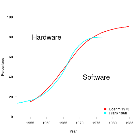
What about the shape of Boehm’s curve? A logistic equation is a possible choice, given just the start/end points, and fitting a regression model finds that  is an almost perfect fit (code+data).
How well does the 1972 prediction agree with 1985 reality?
At the start of the 1980s, two people wrote articles addressing this question: The myth of the hardware/software cost ratio by Harvey Cragon in 1982, and The history of Myth No.1 (page 252) by Werner L. Frank in 1983.
Cragon’s article cites several major ecosystems where recent hardware/software percentage ratios are comparable to Boehm’s ratios from the early 1970s, i.e., no change. Cragon suggests that Boehm’s data applies to a particular kind of project, where a non-recurring cost was invested to develop a new software system either for a single deployment or with more hardware to be purchased at a later date.
When the cost of software is spread over multiple installations, the percentage cost of software can dramatically shrink. It’s the one-of-a-kind developments where software can consume most of the budget.
Boehm’s published a response to Cragon’s article, which answered some misinterpretations of the points raised by Cragdon, and finished by claiming that the two of them agreed on the major points.
The development of software systems was still very new in the 1960s, and ambitious projects were started without knowing much about the realities of software development. It’s no surprise that software costs were so great a percentage of the total budget. Most of Boehm’s articles/reports are taken up with proposed cost reduction ideas, with the hardware/software ratio used to illustrate how ‘unbalanced’ the costs have become, an example of the still widely held belief that hardware costs should consume most of a budget.
Frank’s article references Cragon’s article, and then goes on to spend most of its words citing other articles that are quoting Boehm’s prediction as if it were reality; the second page is devoted 15 plots taken from these articles. Frank feels that he and Boehm share the responsibility for creating what he calls “Myth No. 1” (in a 1978 article, he lists The Ten Great Software Myths).
What happened at the start of 1980, when it was obvious that the software/hardware ratio predicted was not going to happen by 1985? Yes, obviously, move the date of the apocalypse forward; in this case to 1990.
Cragon’s article plots software/hardware budget data from an uncited Air Force report from 1980(?). I managed to find a 1984 report listing more data. Fitting a regression model finds that both hardware and software growth is deemed to be quadratic, with software predicted to consume 84% of DoD budget by 1990 (code+data).
Did software consume 84% of the DoD computer/hardware budget in 1990? Pointers to any subsequent predictions welcome.
My new laptop
I have been using the same MacBook Pro for almost nine years; yes, I’m a sporadic user of laptops, much preferring to work on a decent desktop system. I’ve had zero hardware problems, and have often been able to install programs (often by compiling from source) from the weird and wonderful ecosystems I frequent. Performance does seem to have gotten slower with every OS upgrade (it ‘only’ has 8G of memory). I’m very happy with the eight years of software support provided by Apple; while I’m usually happy to stay with older versions of software, package vendors eventually stop supporting them, ‘forcing’ me to upgrade.
My decision about which laptop to buy next is software driven: Over the next, say, five years which of Apple’s OS X or Linux is most likely to best support the software ecosystems containing the kind of programs I am going to want to run (given a Windows laptop, my first action would be to install the Linux subsystem)?
Diehard Mac fans complain that Apple has lost its way, with regard to Mac upgrades; this does not bother me too much. I am more concerned with the increasing number of features that smack of a walled garden approach to software that is permitted to run on Apple hardware.
My need for a new laptop has not been urgent, and for the last 18-months I have been keeping an eye out for the hardware options that are available for a laptop running Linux.
The most obvious option is buying a Windows laptop from a major supplier, and doing a clean Linux installation; yes, some larger suppliers offer laptops with Linux preinstalled.
About a year ago, I saw a review for the StarBook, which is essentially a hackers’ 14″ laptop built by a bunch of hackers for a living. The hardware specs looked good, with plenty of upgrade options, and choice of preinstalled Linux distribution. While I continue to build desktop systems, I don’t plan to get involved with laptop hardware; however, it’s good to see that Starlab Systems publish complete disassembly instructions.
Around a month ago I finally had had enough with my sluggish MacBook and ordered a StarBook (32G memory, 960G SSD). I initially specified Ubuntu as the installed distribution, but on learning that some Ubuntu tools now produced promotional messages, I switched to Linux Mint.
The StarBook arrived a couple of weeks ago, and is certainly a lot faster than my 2013 MacBook (Geekbench cpu results). There has been the usual period of installing packages and configuring the system (I have yet to spend the time need to figure out how to get Cinnamon (the desktop environment) to save/restore the terminal windows across shutdown (the one OSX feature I miss).
All being well, I may be writing again about my new laptop in 2032.
My MacBook, StarBook and Samsung 32-inch curved monitor. While the laptops have very similar length/width, the screen size of the StarBook is 1-inch greater.
Analysis of a subset of the Linux Counter data
The Linux Counter project was started in 1993, with the aim of tracking the growth of Linux users (the kernel was first released two years earlier). Anybody could register any of their machines running Linux; a user ran a script that gathered basic information about a machine, and the output was emailed to the project. Once registered, users received an annual reminder to update information in their entry (despite using Linux since before the 1.0 release, user #46406 didn’t register until 2001).
When it closed (reopened/closed/coming back) it had 120K+ registered users. That’s a lot of information about computers, which unfortunately is not publicly available. I have not had any replies to my emails to those involved, asking for a copy that could be released in anonymized form.
This week I found 15,906 rows of what looks like a subset of the Linux counter data, most entries are post-2005. What did I learn from this data?
An obvious use is the pattern to check is changes over time. While the data does not include any explicit date, it does include the Kernel version, from which the earliest date can be inferred.
An earlier post used SPEC data to estimate the growth in installed memory over time; it has been doubling every 840 days, give or take. That data contains one data point per distinct vendor computer; the Linux counter data contains one entry per computer in use. There is around thirty pairs of entries for updated systems, i.e., a user updated the entry for an existing system.
The plot below shows memory installed in each registered computer, over time, for servers, laptops and workstations, with fitted regression lines. The memory size doubling times are: servers 4,000 days, laptops 2,000 days, and workstations 1,300 days (code+data):
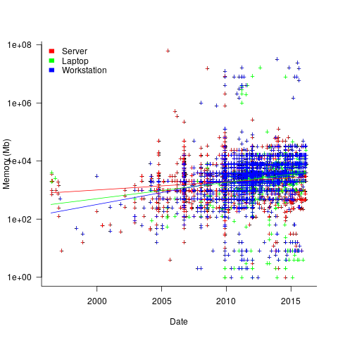
A regression model using dates is a good fit in the statistical sense, but explain very little of the variance in the data. The actual date on which the memory size was selected may have been earlier (because the kernel has been updated to a later release), or later (because memory was added, but the kernel was not updated).
Why is the memory doubling time so long?
Has memory size now reached the big-enough boundary, do Linux counter users keep the same system for many years without upgrading, are Linux counter systems retired Windows boxes that have been repurposed (data on installed memory Windows boxes would answer this point)?
Suggestions welcome.
When memory capacity is limited, it may be useful to swap least recently used memory contents to disc; Linux setup includes the specification of a swap partition. What is the optimal size of the size partition? A common recommendation is: if memory is less than 2G swap size is twice memory; if between 2-8G swap size is the same as memory, and for greater than 8G, half of memory size. The table below shows the percentage of particular system classes having a given swap/memory ratio (rounding the list of ratios to contain one decimal digit produces a list of over 100 ratio values).
swap/memory Server Workstation Laptop 1.0 15.2 19.9 25.9 2.0 10.3 9.6 8.6 0.5 9.5 7.7 8.4 |
The plot below shows memory against swap partition size, for the system classes laptop, server and workstation, with fitted regression line (code+data):
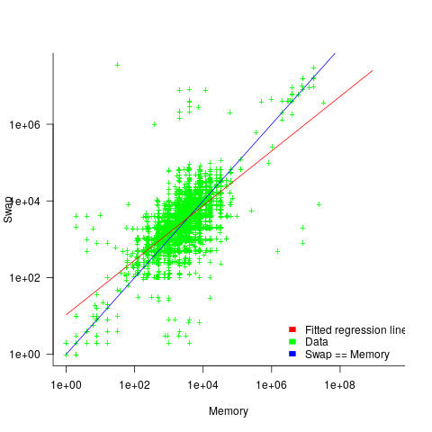
The available disk space also has a (small) impact on swap partition size; the following model explains 46% of the variance in the data:  .
.
I was hoping to confirm the rate of installed memory growth suggested by the SPEC data, with installed systems lagging a few years behind the latest releases. This Linux counter data tells a very different growth story. Perhaps pre-2005 data will tell another story (I just need to find it).
I’m not sure if the swap/memory ratio analysis is of any use to systems people. It was something of a fishing expedition on my part.
Other counting projects have included the Ubuntu counter project, and Hardware for Linux which is still active and goes back to August 2014.
I’m interested in hearing about the availability of any other Linux counter data, or data from other computer counting projects.
Learning useful stuff from the Ecosystems chapter of my book
What useful, practical things might professional software developers learn from the Ecosystems chapter in my evidence-based software engineering book?
This week I checked the ecosystems chapter; what useful things did I learn (combined with everything I learned during all the other weeks spent working on this chapter)?
A casual reader would conclude that software engineering ecosystems involved lots of topics, with little or no theory connecting them. I had great plans for the connecting theories, but lack of detailed data, time and inspiration means the plans remain in my head (e.g., modelling the interaction between the growth of source code written in a particular language and the number of developers actively using that language).
For managers, the usefulness of this chapter is the strategic perspective it provides. How does what they and others are doing relate to everything else, and what patterns of evolution are to be expected?
Software people like to think that everything about software is unique. Software is unique, but the activities around it follow patterns that have been followed by other unique technologies, e.g., the automobile and jet engines. There is useful stuff to be learned from non-software ecosystems, and the chapter discusses some similarities I have learned about.
There is lots more evidence of the finite lifetime of software related items: lifetime of products, Linux distributions, packages, APIs and software careers.
Some readers might be surprised by the amount of discussion about what is now historical hardware. Software needs hardware to execute it, and the characteristics of the hardware of the day can have a significant impact on the characteristics of the software that gets written. I suspect that most of this discussion will not be that useful to most readers, but it provides some context around why things are the way they are today.
Readers with a wide knowledge of software ecosystems will notice that several major ecosystems barely get a mention. Embedded systems is a huge market, as is Microsoft Windows, and very many professional developers use C++. However, to date the focus of most research has been around Linux and Android (because its use of Java, a language often taught in academia), and languages that have a major package repository. So the ecosystems chapter presents a rather blinkered view of software engineering ecosystems.
What did I learn from this chapter?
Software ecosystems are bigger and more complicated that I had originally thought.
Readers might have a completely different learning experience from reading the ecosystems chapter. What useful things did you learn from the ecosystems chapter?
Quality control in a zero cost of replication business
When a new manufacturing material becomes available, its use is often integrated with existing techniques, e.g., using scientific management techniques for software production.
Customers want reliable products, and companies that sell unreliable products don’t make money (and may even lose lots of money).
Quality assurance of manufactured products is a huge subject, and lots of techniques have been developed.
Needless to say, quality assurance techniques applied to the production of hardware are often touted (and sometimes applied) as the solution for improving the quality of software products (whatever quality is currently being defined as).
There is a fundamental difference between the production of hardware and software:
- Hardware is designed, a prototype made and this prototype refined until it is ready to go into production. Hardware production involves duplicating an existing product. The purpose of quality control for hardware production is ensuring that the created copies are close enough to identical to the original that they can be profitably sold. Industrial design has to take into account the practicalities of mass production, e.g., can this device be made at a low enough cost.
- Software involves the same design, prototype, refinement steps, in some form or another. However, the final product can be perfectly replicated at almost zero cost, e.g., downloadable file(s), burn a DVD, etc.
Software production is a once-off process, and applying techniques designed to ensure the consistency of a repetitive process don’t sound like a good idea. Software production is not at all like mass production (the build process comes closest to this form of production).
Sometimes people claim that software development does involve repetition, in that a tiny percentage of the possible source code constructs are used most of the time. The same is also true of human communications, in that a few words are used most of the time. Does the frequent use of a small number of words make speaking/writing a repetitive process in the way that manufacturing identical widgets is repetitive?
The virtually zero cost of replication (and distribution, via the internet, for many companies) does more than remove a major phase of the traditional manufacturing process. Zero cost of replication has a huge impact on the economics of quality control (assuming high quality is considered to be equivalent to high reliability, as measured by number of faults experienced by customers). In many markets it is commercially viable to ship software products that are believed to contain many mistakes, because the cost of fixing them is so very low; unlike the cost of hardware, which is non-trivial and involves shipping costs (if only for a replacement).
Zero defects is not an economically viable mantra for many software companies. When companies employ people to build the same set of items, day in day out, there is economic sense in having them meet together (e.g., quality circles) to discuss saving the company money, by reducing production defects.
Many software products have a short lifespan, source code has a brief and lonely existence, and many development projects are never shipped to paying customers.
In software development companies it makes economic sense for quality circles to discuss the minimum number of known problems they need to fix, before shipping a product.
Performance variation in 2,386 ‘identical’ processors
Every microprocessor is different, random variations in the manufacturing process result in transistors, and the connections between them, being fabricated with more/less atoms. An atom here and there makes very little difference when components are built from millions, or even thousands, of atoms. The width of the connections between transistors in modern devices might only be a dozen or so atoms, and an atom here and there can have a noticeable impact.
How does an atom here and there affect performance? Don’t all processors, of the same product, clocked at the same frequency deliver the same performance?
Yes they do, an atom here or there does not cause a processor to execute more/less instructions at a given frequency. But an atom here and there changes the thermal characteristics of processors, i.e., causes them to heat up faster/slower. High performance processors will reduce their operating frequency, or voltage, to prevent self-destruction (by overheating).
Processors operating within the same maximum power budget (say 65 Watts) may execute more/less instructions per second because they have slowed themselves down.
Some years ago I spotted a great example of ‘identical’ processor performance variation, and the author of the example, Barry Rountree, kindly sent me the data. In the weeks before Christmas I finally got around to including the data in my evidence-based software engineering book. Unfortunately I could not figure out what was what in the data (relearning an important lesson: make sure to understand the data as soon as it arrives), thankfully Barry came to the rescue and spent some time doing software archeology to figure out the data.
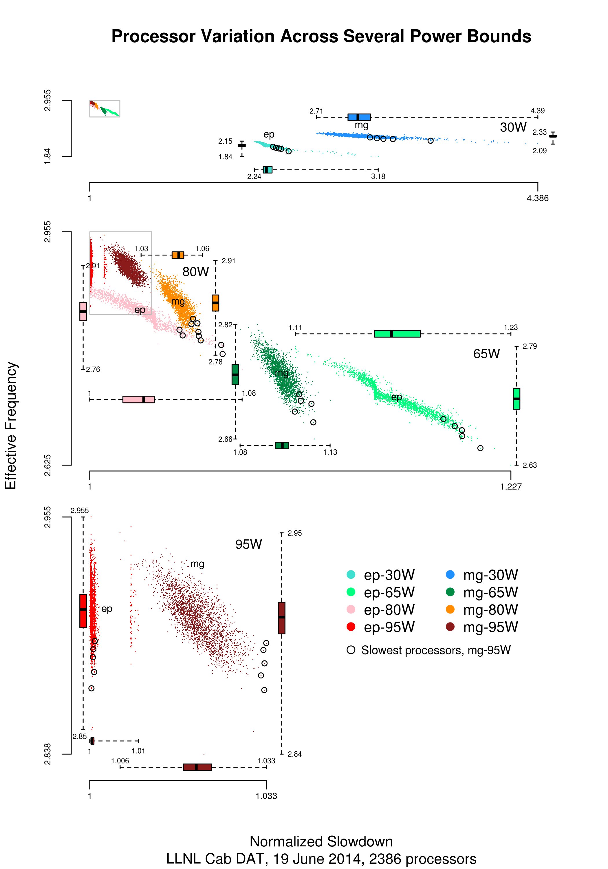
The original plots showed frequency/time data of 2,386 Intel Sandy Bridge XEON processors (in a high performance computer at the Lawrence Livermore National Laboratory) executing the EP benchmark (the data also includes measurements from the MG benchmark, part of the NAS Parallel benchmark) at various maximum power limits (see plot at end of post, which is normalised based on performance at 115 Watts). The plot below shows frequency/time for a maximum power of 65 Watts, along with violin plots showing the spread of processors running at a given frequency and taking a given number of seconds (my code, code+data on Barry’s github repo):
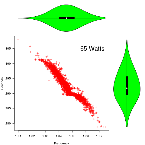
The expected frequency/time behavior is for processors to lie along a straight line running from top left to bottom right, which is roughly what happens here. I imagine (waving my software arms about) the variation in behavior comes from interactions with the other hardware devices each processor is connected to (e.g., memory, which presumably have their own temperature characteristics). Memory performance can have a big impact on benchmark performance. Some of the other maximum power limits, and benchmark, measurements have very different characteristics (see below).
More details and analysis in the paper: An empirical survey of performance and energy efficiency variation on Intel processors.
Intel’s Sandy Bridge is now around seven years old, and the number of atoms used to fabricate transistors and their connectors has shrunk and shrunk. An atom here and there is likely to produce even more variation in the performance of today’s processors.
A previous post discussed the impact of a variety of random variations on program performance.
Update start
A number of people have pointed out that I have not said anything about the impact of differences in heat dissipation (e.g., faster/slower warmer/cooler air-flow past processors).
There is some data from studies where multiple processors have been plugged, one at a time, into the same motherboard (i.e., low budget PhD research). The variation appears to be about the same as that seen here, but the sample sizes are more than two orders of magnitude smaller.
There has been some work looking at the impact of processor location (e.g., top/bottom of cabinet). No location effect was found, but this might be due to location effects not being consistent enough to show up in the stats.
Update end
Below is a png version of the original plot I saw:
Design considerations for Mars colony computer systems
A very interesting article discussing SpaceX’s dramatically lower launch costs has convinced me that, in a decade or two, it will become economically viable to send people to Mars. Whether lots of people will be willing to go is another matter, but let’s assume that a non-trivial number of people decide to spend many years living in a colony on Mars; what computing hardware and software should they take with them?
Reliability and repairability are crucial. Same-day delivery of replacement parts is not an option; the opportunity for Earth/Mars travel occurs every 2-years (when both planets are on the same side of the Sun), and the journey takes 4-10 months.
Given the much higher radiation levels on Mars (200 mS/year; on Earth background radiation is around 3 mS/year), modern microelectronics will experience frequent bit-flips and have a low survival rate. Miniaturization is great for packing billions of transistors into a device, but increases the likelihood that a high energy particle traveling through the device will create a permanent short-circuit; Moore’s law has a much shorter useful life on Mars, compared to Earth. The lesser high energy particles can flip the current value of one or more bits.
Reliability and repairability of electronics, compared to other compute and control options, dictates minimizing the use of electronics (pneumatics is a viable replacement for many tasks; think World War II submarines), and simple calculation can be made using a slide rule or mechanical calculator (both are reliable, and possible to repair with simple tools). Some of the issues that need to be addressed when electronic devices are a proposed solution include:
- integrated circuits need to be fabricated with feature widths that are large enough such that devices are not unduly affected by background radiation,
- devices need to be built from exchangeable components, so if one breaks the others can be used as spares. Building a device from discrete components is great for exchangeability, but is not practical for building complicated cpus; one solution is to use simple cpus, and integrated circuits come in various sizes.
- use of devices that can be repaired or new ones manufactured on Mars. For instance, core memory might be locally repairable, and eventually locally produced.
There are lots of benefits from using the same cpu for everything, with ARM being the obvious choice. Some might suggest RISC-V, and perhaps this will be a better choice many years from now, when a Mars colony is being seriously planned.
Commercially available electronic storage devices have lifetimes measured in years, with a few passive media having lifetimes measured in decades (e.g., optical media); some early electronic storage devices had lifetimes likely to be measured in decades. Perhaps it is possible to produce hard discs with expected lifetimes measured in decades, research is needed (or computing on Mars will have to function without hard discs).
The media on which the source is held will degrade over time. Engraving important source code on the walls of colony housing is one long term storage technique; rather like the hieroglyphs on ancient Egyptian buildings.
What about displays? Have lots of small, same size, flat-screens, and fit them together for greater surface area. I don’t know much about displays, so won’t say more.
Computers built from discrete components consume lots of power (much lower power consumption is a benefit of fabricating smaller devices). No problem, they can double as heating systems. Switching power supplies can be very reliable.
Radio communications require electronics. The radios on the Voyager spacecraft have been operating for 42 years, which suggests to me that reliable communication equipment can be built (I know very little about radio electronics).
What about the software?
Repairability requires that software be open source, or some kind of Mars-use only source license.
The computer language of choice is obviously C, whose advantages include:
- lots of existing, heavily used, operating systems are written in C (i.e., no need to write, and extensively test, a new one),
- C compilers are much easier to implement than, say, C++ or Java compilers. If the C compiler gets lost, somebody could bootstrap another one (lots of individuals used to write and successfully sell C compilers),
- computer storage will be a premium on Mars based computers, and C supports getting close to the hardware to maximise efficient use of resources.
The operating system of choice may not be Linux. With memory at a premium, operating systems requiring many megabytes are bad news. Computers with 64k of storage (yes, kilobytes) used to be used to do lots of useful work; see the source code of various 1980’s operating systems.
Applications can be written before departure. Maintainability and readability are marketing terms, i.e., we don’t really know how to do this stuff. Extensive testing is a good technique for gaining confidence that software behaves as expected, and the test suite can be shipped with the software.
Recent Comments