Archive
Fault density: so costly to calculate that few values are reliable
Fault density (i.e., number of faults per thousand lines of code) often appears in claims relating to software quality.
Fault density sounds like a very useful value to know; unfortunately most quoted values are meaningless and because obtaining reliable data is very costly.
The starting point for calculating fault density is the number of reported faults (I will leave the complexity of what constitutes a line of code for a future post). Most faults don’t get reported.
If there are no reported faults, fault density is zero. The more often software is executed the more likely a fault will be experienced (i.e., the large the range of input values thrown at a program the more likely it will go down a path containing a fault). Comparing like-with-like requires knowing how many different kinds of input a program processed to experience a given number of faults; we don’t want to fall into the trap of claiming heavily used code is less fault prone than lightly used code.
What counts as a fault? One study found that 46% of reported faults in Open Source bug tracking systems were misclassified (e.g., a fault report was actually a request for enhancement). Again, comparing like-with-like requires agreement on what constitutes a fault.
How should faults in code that is no longer shipped be counted? If the current version of a program contains 100K lines and previous versions contained 50K lines that have been deleted, should the faults in those 50K lines contribute to the fault density of the current program? I would say not, which means somebody has to figure out which reported faults apply to code in the current version of the program.
I am aware of less than half a dozen fault density values that I would consider reliable (most calculated during the Rome period). Everything else is little better than reading tea-leafs.
Heartbleed: Critical infrastructure open source needs government funding
Like most vulnerabilities the colorfully named Heartbleed vulnerability in OpenSSL is caused by an ‘obvious’ coding problem of the kind that has been occurring in practically all programs since homo sapiens first started writing software; the only thing remarkable about this vulnerability is its potential to generate huge amounts of financial damage. Some people might say that it is also remarkable that such a serious problem has not occurred in OpenSSL before, I don’t think anybody would describe OpenSSL as the most beautiful of code.
As always happens when a coding problem generates some publicity, there have been calls for:
- More/better training: Most faults are simple mistakes that developers already know all about; training does not stop people making mistakes.
- Switch to a better language: Several lifetimes could be spent discussing this one and a short coffee break would be enough to cover the inconclusive empirical evidence on ‘betterness’. Switching languages also implies rewriting lots of code and there is that annoying issue of newly written code being more likely to contain faults than code that has been heavily used for a long time.
The fact is that all software contains faults and the way to improve reliability is to actively search for and fix these faults. This will cost money and commercial companies have an incentive to spend money doing this; in whose interest is it to fix faults in open source tools such as OpenSSL? There are lots of organizations who would like these faults fixed, but getting money from these organizations to the people who could do the work is going to be complicated. The simple solution would be for some open source programs to be classified as critical infrastructure and have governments fund the active finding and fixing of the faults they contain.
Some people would claim that the solution is to rewrite the software to be more reliable. However, I suspect the economics will kill this proposal; apart from pathological cases it is invariably cheaper to fix what exists that start from scratch.
On behalf of the open source community can I ask that unless you have money to spend please go away and stop bothering us about these faults, we write this code for free because it is fun and fixing faults is boring.
Programming using genetic algorithms: isn’t that what humans already do ;-)
Some time ago I wrote about the use of genetic programming to fix faults in software (i.e., insertion/deletion of random code fragments into an existing program). Earlier this week I was at a lively workshop, Genetic Programming for Software Engineering, with some of the very active researchers in this new subfield.
The genetic algorithm works by having a population of different programs, selecting X% of the best (as measured by some fitness function), making random mutations to those chosen and/or combining bits of programs with other programs; these modified programs are fed back to the fitness function and the whole process iterates until an acceptable solution is found (or a maximum iteration limit is reached).
There are lots of options to tweak; the fitness function gets to decide who has children and is obviously very important, but it can only work with what get generated by the genetic mutations.
The idea I was promoting, to anybody unfortunate enough to be standing in front of me, was that the pattern of usage seen in human written code provides lots of very useful information for improving the performance of genetic algorithms in finding programs having the desired characteristics.
I think that the pattern of usage seen in human written code is driven by the requirements of the problems being solved and regular occurrence of the same patterns is an indication of the regularity with which the same requirements need to be met. As a representation of commonly occurring requirements these patterns are pre-tuned templates for genetic mutation and information to help fitness functions make life/death decisions (i.e., doesn’t look human enough, die!)
There is some noise in existing patterns of code usage, generated by random developer habits and larger fluctuations caused by many developers following the style in some popular book. I don’t have a good handle on estimating the signal to noise ratio.
There has been some work comparing the human maintainability of patches that have been written by genetic algorithms/humans. One of the driving forces behind this work is the expectation that the final patch will still be controlled by humans; having a patch look human-written like is thought to increase the likelihood of it being ‘accepted’ by developers.
Genetic algorithms are also used to improve the runtime performance of programs. Bill Langdon reported that the authors of a program ‘he’ had speeded up by a factor of 70 had not responded to his emails. This may be a case of the authors not knowing how to handle something somewhat off the beaten track; it took a while for Linux developers to start responding to batches of fault reports generated as part of software analysis projects by academic research groups.
One area where human-like might not always be desirable is test case generation. It is easy to find faults in compilers by generating random source code (the syntax/semantics of the randomness follows the rules of the language standard). This approach results in an unmanageable number of fault. Is it worth fixing a fault generated by code that looks like it would never be written by a person? Perhaps the generator should stick to producing test cases that at least look like the code might be written by a person.
Data cleaning: The next step in empirical software engineering
Over the last 10 years software engineering researchers have gone from a state of data famine to being deluged with data. Until recently these researchers have been acting like children at a birthday party, rushing around unwrapping all the presents to see what is inside and quickly moving onto the next one. A good example of this are those papers purporting to have found a power law relationship between two constructs by simply plotting the data using log axis and drawing a straight line through the data; hey look, a power law, isn’t that interesting? Hopefully, these days, reviewers are starting to wise up and insist that any claims of a power law be checked.
Data cleaning is a very important topic that unfortunately appears to be missing from many researchers’ approach to data analysis. The quality of a model built from data is only as good as the quality of the data used to build it. Anybody who is interested in building models that connect to the real world of software engineering, rather than just getting another paper published, has to consider the messiness that gets added to data by the software developers who are intimately involved in the processes that generated the artifacts (e.g., source code, bug reports).
I have jut been reading a paper containing some unsettling numbers (It’s not a Bug, it’s a Feature: On the Data Quality of Bug Databases). A manual classification of over 7,000 issues reported against various large Java applications found that 42.6% of the issues were misclassified (e.g., a fault report was actually a request for enhancement), resulting in a change of status of 39% of the files once thought to contain a fault to not actually containing a fault (any fault prediction models built assuming the data in the fault database was correct now belong in the waste bin).
What really caught my eye about this research was the 725 hours (90 working days) invested by the researchers doing the manual classification (one person + independent checking by another). Anybody can extracts counts of this that and the other from the many repositories now freely available, generate fancy looking plots from them and add in some technobabble to create a paper. Real researchers invest lots of their time figuring out what is really going on.
These numbers are a wakeup call for all software engineering researchers. The data you are using needs to be thoroughly checked and be prepared to invest a lot of time doing it.
Popularity of Open source Operating systems over time
Surveys of operating system usage trends are regularly published and we get to read about how the various Microsoft products are doing and the onward progress of mobile OSs; sometimes Linux gets an entry at the bottom of the list, sometimes it is just ‘others’ and sometimes it is both.
Operating systems are pervasive and a variety of groups actively track reported faults in order to issue warnings to the public; the volume of OS fault informations available makes it an obvious candidate for testing fault prediction models (e.g., how many faults will occur in a given period of time). A very interesting fault history analysis of OpenBSD in a paper by Ozment and Schechter recently caught my eye and I wondered if the fault time-line could be explained by the time-line of OpenBSD usage (e.g., more users more faults reported). While collecting OS usage information is not the primary goal for me I thought people would be interested in what I have found out and in particular to share the OS usage data I have managed to obtain.
How might operating system usage be measured? Analyzing web server logs is an obvious candidate method; when a web browser requests information many web servers write information about the request to a log file and this information sometimes includes the name of the operating system on which the browser is running.
Other sources of information include items sold (licenses in Microsoft’s case, CDs/DVD’s for Open source or perhaps books {but book sales tend not to be reported in the way programming language book sales are reported}) and job adverts.
For my time-line analysis I needed OpenBSD usage information between 1998 and 2005.
The best source of information I found, by far, of Open source OS usage derived from server logs (around 138 million Open source specific entries) is that provided by Distrowatch who count over 700 different distributions as far back as 2002. What is more Ladislav Bodnar the founder and executive editor of DistroWatch was happy to run a script I sent him to extract the count data I was interested in (I am not duplicating Distrowatch’s popularity lists here, just providing the 14 day totals for OS count data). Some analysis of this data below.
As luck would have it I recently read a paper by Diomidis Spinellis which had used server log data to estimate the adoption of Open Source within organizations. Diomidis researches Open source and was willing to run a script I wrote to extract the User Agent string from the 278 million records he had (unfortunately I cannot make this public because it might contain personal information such as email addresses, just the monthly totals for OS count data, tar file of all the scripts I used to process this raw log data; the script to try on your own logs is countos.sh).
My attempt to extract OS names from the list of User Agent strings Diomidis sent me (67% of of the original log entries did contain a User Agent string) provides some insight into the reliability of this approach to counting usage (getos.awk is the script to try on the strings extracted with the earlier script). There is no generally agreed standard for:
- what information should be present; 6% of UA strings contained no OS name that I knew (this excludes those entries that were obviously robots/crawlers/spiders/etc),
- the character string used to specify a given OS or a distribution; the only option is to match a known list of names (OS names used by Distrowatch,
missos.awkis the tar file script to print out any string not containing a specified list of OS names, the Wikipedia List of operating systems article), - quality assurance; some people cannot spell ‘windows’ correctly and even though the source is now available I don’t think anybody uses CP/M to access the web (at least 91 strings,
 %, would not have passed).
Ladislav Bodnar thinks that log entries from the same IP addresses should only be counted once per day per OS name. I agree that this approach is much better than ignoring address information; why should a person who makes 10 accesses be counted 10 times, a person who makes one access is only counted once. It is possible that two or more separate machines running the same OS are accessing the Internet through a common gateway that results in them having the IP address from an external server’s point of view; this possibility means that the Distrowatch data undercounts the unique accesses (not a serious problem if most visitors have direct Internet access rather than through a corporate network).
The Distrowatch data includes counts for all IP address and from 13 May 2004 onwards unique IP address per day per OS. The mean ratio between these two values, summed over all OS counts within 14 day periods, is 1.9 (standard deviation 0.08) and the Pearson correlation coefficient between them is 0.987 (95% confidence interval is 0.984 to 0.990), i.e., almost perfect correlation.
The Spinellis data ignores IP address information (I got this dataset first, and have already spent too much time collecting to do more data extraction) and has 10 million UA strings containing Open source OS names (6% of all OS names matched).
How representative are the Distrowatch and Spinellis data? The data is as representative of the general OS population as the visitors recorded in the respective server logs are representative of OS usage. The plot below shows the percentage of visitors to Distrowatch that use Ubuntu, Suse, Redhat. Why does Redhat, a very large company in the Open source world, have such a low percentage compared to Ubuntu? I imagine because Redhat customers get their updates from Redhat and don’t see a need to visit sites such as Distrowatch; a similar argument can be applied to Suse. Perhaps the Distrowatch data underestimates those distributions that have well known websites and users who have no interest in other distributions. I have not done much analysis of the Spinellis data.
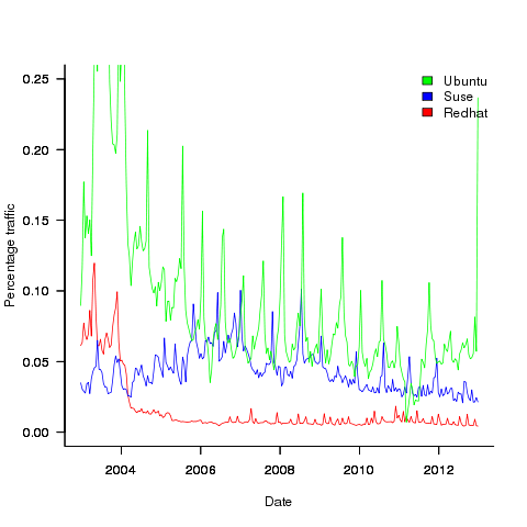
Presumably the spikes in usage occur around releases of new versions, I have not checked.
For my analysis I am interested in relative change over time, which means that representativeness and not knowing the absolute number of OSs in use is not a problem. Researchers interested in a representative sample or estimating the total number of OSs in use are going to need a wider selection of data; they might be interested in the following OS usage information I managed to find (yes I know about Netcraft, they charge money for detailed data and I have not checked what the Wayback Machine has on file):
- Wikimedia has OS count information back to 2009. Going forward this is a source of log data to rival Distrowatch’s, but the author of the scripts probably ought to update the list of OS names matched against,
- w3schools has good summary data for many months going back to 2003,
- statcounter has good summary data (daily, weekly, monthly) going back to 2008,
- TheCounter.com had data from 2000 to 2009 (csv file containing counts obtained from Wayback Machine).
If any reader has or knows anybody who has detailed OS usage data please consider sharing it with everybody.
Low defect density implies climate code less, not more, reliable
I have just been reading a paper comparing the defect density of three climate modelling systems against software from other application domains. The defect density (total reported defects divided by thousands of lines of code) of the climate modelling software was significantly lower than everything else, leading the researchers to conclude that “… suggests that the models are of high software quality,”. I would draw the opposite conclusion, the models have low reliability (I have no idea what software quality is and avoid using the term).
I don’t disagree with Pipitone and Easterbrook numbers, just their conclusion.
There is a very simple technique for creating software that has a low defect density, don’t try too hard to look for defects. There are two reasons why I think this has happened with the climate model software:
- Three of the non-climate systems compared against were the Apache HTTP demon, the VTK visulalization toolkit and the Eclipse project. These are all widely used projects with many thousands of users, millions for Apache; this volume of usage corresponds to a huge amount of testing, and it is no wonder that so many faults have been reported. Each climate model tends to be used by one site, a tiny amount of testing, and it is not surprising that few faults have been reported.
- Climate models have a big intrinsic testing problem; what is the result of a test supposed to be? With applications such as word processors, browsers, compilers, operating systems, etc the expected behavior is known in many cases so it is possible to write test cases that check for the expected behavior. How does anybody know what the expected behavior of a climate model is? If all the climate models did was to solve the Navier-Stokes equation on a rotating sphere there would be no need for multiple models and the UK Meteorological Office’s Unified model would not have grown from 100 KLOC to 800+ KLOC over the last 15 years.
The one system having a similar defect density to the climate models that Pipitone and Easterbrook compare against is an air traffic control system developed using formal methods, exactly the kind of (expensive and time-consuming) development process that one would expect to have a low defect density.
Software is remarkably fault-tolerant and so, yes, serious fault could exist in the climate models and they would still give answers that looked about right. Based on his experience working on a meteorological model Les Hatton tells the story of a fault so serious that the answers should be completely wrong, but they were not.
If somebody wants to convince me that the software in any of these climate models really is reliable then I want to know about the test suites used to check the behavior; what coverage of the source does the suite have (a high MC/DC would be very good, but I would settle for a very high statement coverage) and how were the expected behaviors calculated.
Distribution of uptimes for high-performance computing systems
Computers break down every now and again and this is a serious problem when an application needs runs on thousands of individual computers (nodes) plugged together; lots more hardware creates lots more opportunity for a failure that renders any subsequent calculations by working nodes possible wrong. The solution is checkpointing; saving the state of each node every now and again, and rolling back to that point when a failure occurs. Picking the optimal interval between checkpoints requires knowledge the distribution of node uptimes, what is it?
Short answer: Node uptimes have a negative binomial distribution, or at least five systems at the Los Alamos National Laboratory do.
The longer answer is below as another draft section from my book Empirical software engineering with R. As always comments and pointers to more data welcome. R code and data here.
Distribution of uptimes for high-performance computing systems
Today’s high-performance computing systems are created by connecting together lots of cpus. There is a hierarchy to the connection in that many cpus may populate a single board, several boards may be fitted into a rack unit, several rack units into a cabinet, lots of cabinets lined up in a row within a room and more than one room in a facility. A common operating unit is the node, effectively a computer on which an operating system is running (the actual hardware involved may be a single or multi processor cpu). A high-performance system is built from thousands of nodes and an application program may run on compute nodes from more than one facility.
With so many components, failures occur on a regular basis and long running applications need to recover from such failures if they are to stand a reasonable chance of ever completing.
Applications running on the systems installed at the Los Alamos National Laboratory create checkpoints at regular intervals, writing data needed to do a full restore to storage. When a failure occurs an application is restarted from its most recent checkpoint, one node failure causes all nodes to be rolled back to their most recent checkpoint (all nodes create their checkpoints at the same time).
A tradeoff has to be made between frequently creating checkpoints, which takes resources away from completing execution of the application but reduces the amount of lost calculation, and infrequent checkpoints, which diverts less resources but incurs greater losses when a fault occurs. Calculating the optimum checkpoint interval requires knowing the distribution of node uptimes and the following analysis attempts to find this distribution.
Data
The data comes from 23 different systems installed at the Los Alamos National Laboratory (LANL) between 1996 and 2005. The total failure count for most of the systems is of the order of a few hundred; there are five systems (systems 2, 16, 18, 19 and 20) that each have several thousand failures and these are the ones analysed here.
The data consists of failure records for every node in a system. A failure record includes information such as system id, node number, failure time, restored to service time, various hardware characteristics and possible root causes for the failure. Schroeder and Gibson <book Schroeder_06> performed the first analysis of the dataset and provide more background details.
Is the data believable?
Failure records are created by operations staff when they are notified by the automated monitoring system that a failure has been detected. Given that several people are involved in the process <book LANL_data_06> it seems unlikely that failures will go unreported.
Some of the failure reports have start times before the given node was returned into service from the previous failure; across the five systems this varied between 0.4% and 2.5%. It is possible that these overlapping failures are caused by an incorrectly attempt to fix the first failure, or perhaps they are data entry errors. This error rate is comparable with human error rates for low stress/non-critical work
The failure reports do not include any information about the application software running on the node when it failed; the majority of the programs executed are large-scale scientific simulations, such as simulations of nuclear stockpile stability. Thus it is not possible to accurately calculate the node MTBF for an executing application. LANL say <book LANL_data_06> that the applications “… perform long periods (often months) of CPU computation, interrupted every few hours by a few minutes of I/O for check-pointing.”
Predictions made in advance
The purpose of this analysis is to find the distribution that best fits the node uptime data, i.e., the time interval between failures of the same node.
Your author is not aware of any empirically based theory that predicts the uptime of high performance computing systems. The Poisson and exponential distributions are both frequently encountered in the analysis of hardware failures and it is always comforting to fit in with existing expectations.
Applicable techniques
A [Cullen and Frey test] matches a dataset’s skew and kurtosis against known distributions (in the case of the descdist function in the fitdistrplus package this is a handful of commonly encountered distributions); the fitdist function in the same package can be used to fit the data to a specified distribution.
Results
The table below lists some basic properties of each of the systems analysed. The large difference in mean/median uptimes between some systems is caused by very fat tails in the uptime distribution of some systems, see [LANL-node-uptime-binned].
| System | Nodes | Failures | Mean | Median |
|---|---|---|---|---|
|
2
|
49
|
6997
|
133
|
377
|
|
16
|
16
|
2595
|
89
|
229
|
|
18
|
823
|
3014
|
2336
|
4147
|
|
19
|
738
|
2344
|
2376
|
4069
|
|
20
|
323
|
2063
|
653
|
2544
|
If there are any significant changes in failure rate over time or across different nodes in a given system it could have a significant impact on the distribution of uptime intervals. So we first check to large differences in failure rates.
Do systems experience any significant changes in failure rate over time?
The plot below shows the total number of failures, binned using 30-day periods, for the five systems. Two patterns that stand out are system 20 which experienced many failures during the first few months and then settled down, and system 2’s sudden spike in failures around month 23 before settling down again. This analysis is intended to be broad brush and does not get involved with details of specific systems, but these changes in failure frequency suggest that the exact form of any fitted distribution may change over time in turn potentially leading to a change of checkpoint interval.
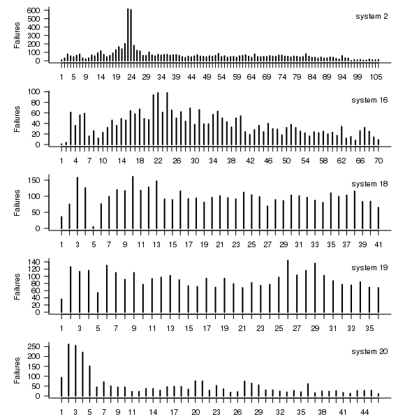
Figure 1. Total number of failures per 30-day interval for each LANL system.
Do some nodes failure more often than others?
The plot below shows the total number of failures for each node in the given system. Node 0 has many more failures than the other nodes (for node 0 of system 2 most of the failure data appears to be missing, so node 1 has the most failures). The distribution suggested by the analysis below is not changed if Node 0 is removed from the dataset.
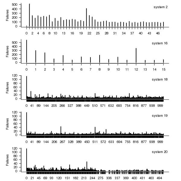
Figure 2. Total number of failures for each node in the given LANL system.
Fitting node uptimes
When plotted in units of 1 hour there is a lot of variability and so uptimes are binned into 10 hour units to help smooth the data. The number of uptimes in each 10-hour bin forms a discrete distribution and a [Cullen and Frey test] suggests that the negative binomial distribution might provide the best fit to the data; the Scroeder and Gibson analysis did not try the negative binomial distribution and of those they tried found the Weilbull distribution gave the best fit; the R functions were not able to fit this distribution to the data.
The plot below shows the 10-hour binned data fitted to a negative binomial distribution for systems 2 and 18. Visually the negative binomial distribution provides the better fit and the Akaiki Information Criterion values confirm this (see code for details and for the results on the other systems, which follow one of the two patterns seen in this plot).
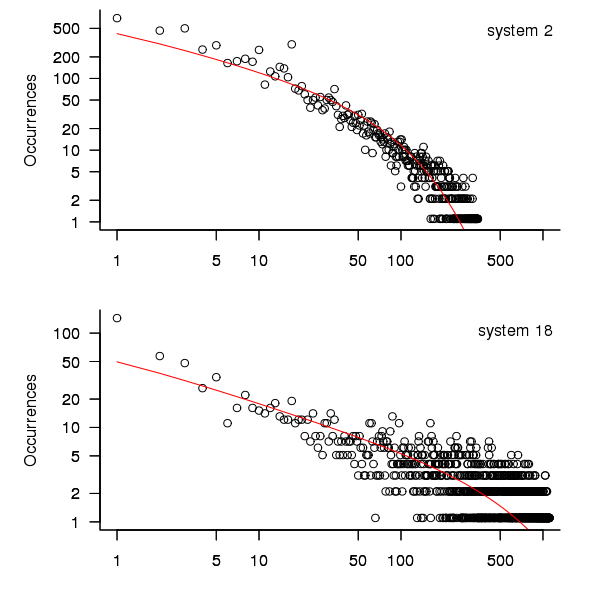
Figure 3. For systems 2 and 18, number of uptime intervals, binned into 10 hour interval, red line is fitted negative binomial distribution.
The negative binomial distribution is also the best fit for the uptime of the systems 16, 19 and 20.
The Poisson distribution often crops up in failure analysis. The quality of fit of a Poisson distribution to this dataset was an order of worse for all systems (as measured by AIC) than the negative binomial distribution.
Discussion
This analysis only compares how well commonly encountered distributions fit the data. The variability present in the datasets for all systems means that the quality of all fitted distributions will be poor and there is no theoretical justification for testing other, non-common, distributions. Given that the analysis is looking for the best fit from a chosen set of distributions no attempt was made to tune the fit (e.g., by forming a zero-truncated distribution).
Of the distributions fitted the negative binomial distribution has the lowest AIC and best fit visually.
As discussed in the section on [properties of distributions] the negative binomial distribution can be generated by a mixture of [Poisson distribution]s whose means have a [Gamma distribution]. Perhaps the many components in a node that can fail have a Poisson distribution and combined together the result is the negative binomial distribution seen in the uptime intervals.
The Weilbull distribution is often encountered with datasets involving some form of time between events but was not seen to be a good fit (for a continuous distribution) by a Cullen and Frey test and could not be fitted by the R functions used.
The characteristics of node uptime for two systems (i.e., 2 and 16) follows what might be thought of as a typical distribution of measurements, with some fattening in the tail, while two systems (i.e., 18 and 19) have very fat tails with indeed and system 20 sits between these two patterns. One system characteristic that matches this pattern is the number of nodes contained within it (with systems 2 and 16 having under 50, 18 and 19 having over 1,000 and 20 having around 500). The significantly difference in the size of the tails is reflected in the mean uptimes for the systems, given in the table above.
Summary of findings
The negative binomial distribution, of the commonly encountered distributions, gives the best fit to node uptime intervals for all systems.
There is over an order of magnitude variation in the mean uptime across some systems.
Impact of compiler optimization level on recovery from a hardware error
I have previously written about cosmic-ray induced faults in cpus and some of the compiler research being done to recover from such hardware faults. If your program is executing in an environment where radiation may cause hardware bit-flips to occur and you don’t have access to a research compiler providing some level of recovery, is it better to compile with high or low levels of optimization?
Short answer: Using gcc with optimization options O2 or O3 reduces the probability that a bit-flip will change the external behavior of a program, compared to option O0.
The longer answer is below as another draft section from my book Empirical software engineering with R book. As always comments welcome.
Software masking of hardware faults
Like all hardware cpus are subject to intermittent faults, these faults may flip the value of a bit in a program visible register, a bit in an executable instruction or some internal processor state (causes include cosmic rays, and electrical wear of the material from which circuits are built).
If a bit-flip randomly occurs at some point during a program’s execution, is it less likely to effect external program behavior when the code has been built with high levels of compiler optimization or built with optimization disabled or at a low level?
- many optimizations reduce the number of instructions executed (reducing execution time reduces the probability of encountering a bit-flip) and makes more efficient use of registers (e.g., keeping needed values in registers over longer periods of time and reducing the time intervals when a registers is not in use; which increases the probability that a bit-flip will propagate to external behavior),
- fewer compiler optimizations is likely to result in an increased number of instructions executed (increasing the probability that a bit-flip will occur during program execution) and results in lower register usage efficiency (e.g., longer periods of time between the last use of register contents and a new value being loaded; increasing the probability that a bit-flip will modify a value that is never used again).
A study by Cook and Zilles flipped one bit in an executing program (100 evenly distributed points in the program were chosen and 100 instructions from each of those points were used as fault injection points, giving a total of 10,000 individual tests to be run) and monitored the impact on subsequent execution; this process was repeated between 32 and 244 times for each injection point, once for every bit in the 32-bit instruction, zero, one or two of its 64-bit input registers and one possible 64-bit output result register (i.e., the bit-flip only involved the current instruction and its input/output, not the contents of any other register or main memory).
The monitoring process consisted of two parallel executions containing the modified processor state and the unmodified processor state. The behavior of the two executions were compared to see if the fault did not propagate (a passing trial, e.g., a bit-wise AND of a register with 0xff when a bit-flip has been applied to one of the top 24 bits of the register, also the values in a branch not-equal are usually not-equal and a bit-flip is likely to maintain that state), caused a failure (either due to a compulsory event caused by a hardware trap such as an invalid instruction or an incorrectly aligned memory access, or what was called an error model event such as a control flow mismatch or writing a different value to storage), or is inconclusive (pass/fail did not occur within 10,000 executed instructions of the fault injection point).
Data
The available data consists of the normalised number of program executions having one of the behaviors pass, fail (compulsory), fail (error model, broken down into control flow and store related cases) or inconclusive for nine programs from the SPEC2000 integer benchmark compiled using gcc version 4.0.2 and the DEC C compiler (henceforth called O0, O2 and O3, for osf the O4 option was used.
There are nine measurements for each of the nine SPEC programs, repeated at 3 optimization levels for gcc and once for osf (the osf data is not analysed here).
Is the data believable?
Injecting bit-flip faults at all points in a program and monitoring for subsequence changes in external behavior would be an enormous task, sets of 100 instructions starting from 100 locations appears to be an unbiased sample.
The error model used checks for changes of control flow and different values being stored to memory, it does not check for actual changes in external program behavior. This model biases the measurements in favour of more bit-flips being counted as generating an error than would occur in practice.
Predictions made in advance
Does compiler optimization level change the probability that a bit-flip will cause a change in external program behavior?
No hypothesis is proposed suggesting that compiler optimization level will increase, decrease or have no effect on the probability of a bit-flip effecting external program behavior.
Applicable techniques
The data was originally a count of the number of instances and this has been normalised to a value between 0 and 100. The same number of programs were executed at all optimization levels.
Non-parametric techniques have to be used because nothing is known about the distribution of values.
The [Wilcoxon signed-rank test] is a test for two dependent samples while the [Mann-Whitney U test] is a test for two independent samples. To what extent does running gcc at different optimization levels make it a different compiler? Given that we are testing for the possibility that compiler optimizations do effect the results then it is necessary to treat the samples as being independent.
The function wilcox.test will perform a Mann-Whitney test if the parameter paired is FALSE (the default) and will generate a confidence interval if the parameter conf.int is TRUE (the default is FALSE).
Results
The Mann-Whitney test of the various measurements obtained using the O2 and O3 options finds no worthwhile difference between them. There are interesting differences in the values obtained using both of two options and the O0 option, as follows:
- Pass
-
Comparing percentage of pass behaviors for
O0andO2we see: p-values = 0.005 and 0.005
> wilcox.test(gcc.o0$pass.masked, gcc.o2$pass.masked, conf.int=TRUE)
        Wilcoxon rank sum test with continuity correction

data:  gcc.o0$pass.masked and gcc.o2$pass.masked
W = 8, p-value = 0.004697
alternative hypothesis: true location shift is not equal to 0
95 percent confidence interval:
 -15.449995  -2.020001
sample estimates:
difference in location
             -7.480088
The wilcox.test function returns an estimate of the difference between the two means and a negative value occurs if the second argument (the higher optimization level in this case) has a greater mean than the first argument (which is always the O0 option in these results).
O0/O3 95% confidence interval: -15.579959 -1.909965, mean: -4.780058
- Fail (compulsory)
-
-
Memory protection fault: pvalues = 0.002 and 0.005
O0/O295%: 2.1 7.5, mean: 4.9
O0/O395%: 1.9 7.3, mean: 4.1 -
Invalid instruction: p-values = 0.045 and 0.053
O0/O295%: -8.0e-01 -4.9e-08, mean: -0.5
O0/O395%: -6.4e-01 5.1e-06, mean: -0.3
-
Memory protection fault: pvalues = 0.002 and 0.005
- Fail (error model)
-
-
Control flow: p-values = 0.0008 and 0.002
O0/O295%: -10.8 -3.8, mean: -7.0
O0/O395%: -10.5 -3.7, mean: -6.8 -
Store related: p-values = 0.002 and 0.003
O0/O295%: 4.78 22.02, mean: 11.24
O0/O395%: 4.93 18.78, mean: 10.51
-
Control flow: p-values = 0.0008 and 0.002
Discussion
O2 and O3 options differences
The issue of optimization performance differences between the gcc O2 and O3 options is covered in [another section] of this book. That analysis found that the only difference between the two options was an increase in code size with O3, probably because of function inlining.
If there is no significant difference in the code generated by the O2/O3 options then no difference in bit-flip behavior is expected, and none was seen.
Changes in failure rates
The results show a decrease in store related errors at high optimization levels and an increase in control flow related errors. Why is this?
Optimizing register usage is a very important optimization and one of its consequences is a reduction in the number of stores to memory and loads having a corrupted address triggering a protection fault . A reduction in the number of memory related instructions executed will feed through into a reduction in the number of failures classified as store related or memory protection faults and this is seen in the shift in mean value of fails between high and low optimization levels.
Keeping a value containing an injected bit-flip in a register for a longer period of program execution (rather than being stored to memory and loaded back later) provides the opportunity for it to work its way through subsequent instructions and either disappear (being counted as a pass) or cause a control flow failure. It is likely that some of the change stored values flagged by the error model do not an impact on external program behavior and the pass count at low optimization levels is lower than would occur in practice.
Changes in pass rate
The additional optimizations of register usage enabled by the O2/O3 options reduces memory accesses which leads to a reduction in memory protection errors, an unrecoverable fault under all circumstances. The numbers suggest that while this is a major factor in the increased pass rate, contributions are made by other sources, e.g., bit-flips not contributing to the result calculated by an instruction; the data is not sufficiently detailed to enable a reliable estimate of this contribution to be made.
The pass rate is likely to be an underestimate because the error model classifies storing a different value as a failure, however the different value might not result in a change of external program behavior, e.g., the value stored might never be used again. Some of the stores classified as errors for the O0 option have no lasting affect in practice (and being kept in registers for O2/O3 had the opportunity to be masked out). No data is available for enable an estimate to be made for the percentage of these bit-flips have no lasting affect.
The average pass rate for gcc using the O0 option was 28% and this increased to around 36% when the O2/O3 options were used.
Other processors
How likely is it that the bit-flip pass rates seen on the Alpha (average of 36% for high optimization, 28% for low) would also occur on other processors?
The Alpha registers contain 64-bit and instructions operating on just 32 or 16 of those bits are supported. A study by Loh of the Alpha running SPEC2000 programs found that 48% of executed instructions operated on 64-bits, 24% on 32-bits and 28% on 16-bits. Based on these numbers 33% of single bit-flips of a 64-bit register would not be expected to affect the result of an instruction (the table below gives the percentages measured by Cook et al).
| injection site | O3 | O2 | O0 |
|---|---|---|---|
|
instruction
|
28.2
|
29.2
|
21.3
|
|
input register1
|
49.0
|
50.0
|
40.5
|
|
input register2
|
26.5
|
28.5
|
17.9
|
|
output register
|
39.6
|
41.9
|
34.7
|
A lot of software is based on using 32-bit integers and it might be expected that a much lower percentage of register bit-flips would result in pass behavior, compared to a 64-bit processor (where most operations that access 64 bits involve addresses). However, 32-bit processors usually contain instructions for operating on just 8-bits of a register and use of these instructions creates more opportunities for bit-flips to have no lasting consequences.
The measurements of Cook and Zilles have shown how interrelated instruction set interactions are. Without measurements from 32-bit processors it is not possible to estimate the extent to which bit-flips will impact external program behavior.
Conclusion
Compiling source using high levels of compiler optimization reduces the likelihood that a randomly occurring bit-flip during program execution will effect external program behavior. For processors that perform memory access checks the largest decrease in bit-flip induced faults is a reduction in memory protection faults.
Optimization generally reduces the number of instructions executed by a program, reducing the probability that a bit-flip will occur between the start and end of execution, further increasing the advantage of optimized code over non-optimized.
Undefined behavior can travel back in time
The committee that produced the C Standard tried to keep things simple and sometimes made very short general statements that relied on compiler writers interpreting them in a ‘reasonable’ way. One example of this reliance on ‘reasonable’ behavior is the definition of undefined behavior; “… erroneous program construct or of erroneous data, for which this International Standard imposes no requirements”. The wording in the Standard permits a compiler to process the following program:
int main(int argc, char **argv) { // lots of code that prints out useful information 1 / 0; // divide by zero, undefined behavior } |
to produce an executable that prints out “yah boo sucks”. Such behavior would probably be surprising to the developer who expected the code printing the useful information to be executed before the divide by zero was encountered. The phrase quality of implementation is heard a lot in committee discussions of this kind of topic, but this phrase does not appear in any official document.
A modern compiler is essentially a sophisticated domain specific data miner that happens to produce machine code as output and compiler writers are constantly looking for ways to use the information extracted to minimise the code they generate (minimal number of instructions or minimal amount of runtime). The following code is from the Linux kernel and its authors were surprised to find that the “division by zero” messages did not appear when arg2 was 0, in fact the entire if-statement did not appear in the generated code; based on my earlier example you can probably guess what the compiler has done:
if (arg2 == 0) ereport(ERROR, (errcode(ERRCODE_DIVISION_BY_ZERO), errmsg("division by zero"))); /* No overflow is possible */ PG_RETURN_INT32((int32)arg1 / arg2); |
Yes, it figured out that when arg2 == 0 the divide in the call to PG_RETURN_INT32 results in undefined behavior and took the decision that the actual undefined behavior in this instance would not include making the call to ereport which in turn made the if-statement redundant (smaller+faster code, way to go!)
There is/was a bug in Linux because of this compiler behavior. The finger of blame could be pointed at:
- the developers for not specifying that the function
ereportdoes not return (this would enable the compiler to deduce that there is no undefined behavior because the divide is never execute whenarg2 == 0), - the C Standard committee for not specifying a timeline for undefined behavior, e.g., program behavior does not become undefined until the statement containing the offending construct is encountered during program execution,
- the compiler writers for not being ‘reasonable’.
In the coming years more and more developers are likely to encounter this kind of unexpected behavior in their programs as compilers do more and more data mining and are pushed to improve performance. Other examples of this kind of behavior are given in the paper Undefined Behavior: Who Moved My Code?
What might be done to reduce the economic cost of the fallout from this developer ignorance/standard wording/compiler behavior interaction? Possibilities include:
- developer education: few developers are aware that a statement containing undefined behavior can have an impact on the execution of code that occurs before that statement is executed,
- change the wording in the Standard: for many cases there is no reason why the undefined behavior be allowed to reach back in time to before when the statement executing it is executed; this does not mean that any program output is guaranteed to occur, e.g., the host OS might delete any pending output when a divide by zero exception occurs.
- paying gcc/llvm developers to do front end stuff: nearly all gcc funding is to do code generation work (I don’t know anything about llvm funding) and if the US Department of Homeland security are interested in software security they should fund related front end work in gcc and llvm (e.g., providing developers with information about suspicious usage in the code being compiled; the existing
-Wallis a start).
Why do companies fix faults in software they sell?
Once I buy some software from a company they have my money, if sometime later I find a fault software what incentive does that company have to fix the software and provide me with an update (assuming the software is not so fault ridden that I take advantage of laws allowing me to return a purchase for a refund)?
There are three economic incentives for companies to fix faults:
- because I am paying them a fee for updates that include fixes to known faults,
- because they want to make future sales to me and to others (faults encountered by customers contribute towards the perception of product quality),
- they don’t want to lose money because a fault had consequences that resulted in legal action (this reason is overhyped, in practice software engineering has a missing dead body problem).
Which faults get fixed? Software is surprisingly fault-tolerant and there is no point in fixing faults that customers are unlikely to encounter. This means that once a product has been released and known to be acceptable to many customers, there is no incentive to actively search for faults; this means that the only faults likely to be fixed are the ones reported by customers.
When reporting a fault, customers are often asked to rate its severity. This is a useful technique for prioritizing what gets fixed first, or perhaps what does not get fixed at all. Customers who actively set out to find faults are not appreciated and are labelled as disruptive if they continue doing it. Finding faults is surprisingly easy, finding the faults that have a high probability of being encountered by customers and ranked by them as critical is very hard (this is one of the reasons static analysis tools are not widely used).
What is the motivation for developers to fix faults in Open Source?
- There are companies who provide support services for a fee, just like commercial offerings,
- Open Source is free, gaining more users is not an obvious incentive to fix faults. However, being known as the go-to guys for a given package is a way of attracting companies looking to hire somebody to provide support services or make custom modifications to that package. Fixing faults is a way of getting visibility, it is advertising.
- Developers hate the thought of doing something wrong resulting in a fault in code they have written, and writing faulty code is not socially acceptable behavior in software development circles. These feelings about what constitutes appropriate behavior are often enough to make developers want to spend time fixing faults in code they have written or feel responsible for, provided they have the time. I suspect a lot of faults get fixed by developers when their manager/wife thinks they are working on something more ‘useful’.
Recent Comments