Archive
Measuring non-determinism in the Linux kernel
Developers often assume that it’s possible to predict the execution path a program will take, for a given set of input values, i.e., program behavior is deterministic. The execution path may be very complicated, and may depend on the contents of certain files (e.g., SQL engines), but it’s deterministic.
There is one kind of program where determinism is not an option; operating systems are non-deterministic when running in a mode where interrupts can occur.
How much non-determinism can occur in, say, Linux? For instance, when a program calls a system function (e.g., open, read, write, close), how often does the execution sequence follow the function call tree that appears in the source code, and how many different call sequences actually occur during program execution (because of diversions caused by an interrupt; ignoring control flow within functions)?
A study by Imanol Allende ran the same program 500K+ times, and traced every function call that occurred within the Linux kernel (thanks to Imanol for sending me the data and answering my questions). The program used appears below; the system calls traced were open (two distinct calls), read, write, and close (two distinct calls); a total of six system calls.
// #includes omitted int main(int argc, char **argv) { unsigned char result; int fd1, fd2, ret; char res_str[10]={0}; fd1 = open("/dev/urandom", O_RDONLY); fd2 = open("/dev/null", O_WRONLY); ret = read(fd1 , &result, 1); sprintf(res_str ,"%d", result); ret = write(fd2, res_str, strlen(res_str)); close(fd1); close(fd2); return ret; } |
Analysing each of these six distinct calls, in around 98% of program runs, each call follows the same sequence of function calls within the kernel (the common case for write involves a chain of around 10 function calls). During the other 2’ish% of calls, the common sequence was interrupted for some reason, and the logged call trace includes additional called functions, e.g., calls involving the Read, Copy, Update synchronization mechanism. The plot below shows the growth in the number of unique traces against the number of program runs (436,827 of them) for the close(fd2) call; a fitted regression line is in red, with the first 1,000 runs not included in the fit (code+data):
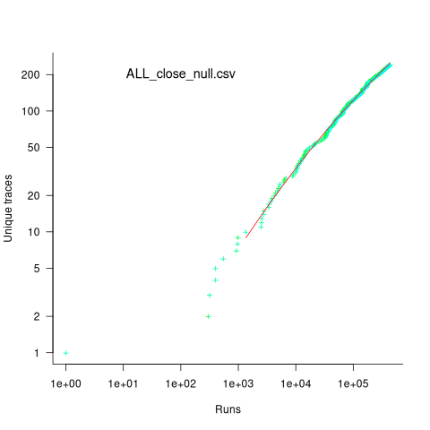
The fitted regression model is ^2") , suggesting that the growth in unique traces is slowing (this equation peaks at around
, suggesting that the growth in unique traces is slowing (this equation peaks at around  ), while the model fitted to some of the system calls implies ever continuing growth.
Allende investigated more sophisticated techniques for estimating the total number of unique traces, including: extreme value theory and species estimation techniques from ecology.
While around 98% of traces are the common case, over half of the unique traces occurred once in 436,827 runs. The plot below shows the number of occurrences of each unique trace, for the close(fd2) call, with an attempted fit of a bi-exponential model (in red; code+data):
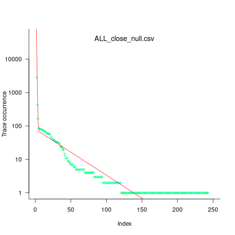
The analysis above looked at one system call, the program contains six system calls. If, for each system call, the probability of the most common trace is 98%, then the probability of all six calls following their respective common case is 89%. As the number of distinct system calls made by a program goes up, the global common case becomes less common, and the number of distinct program traces increases multiplicatively.
A surprising retrospective task estimation dataset
When estimating the time needed to implement a task, the time previously needed to implement similar tasks provides useful guidance. The implementation time for these previous tasks may itself be estimated, because the actual time was not measured or this information is currently unavailable.
How accurate are developer time estimates of previously completed tasks?
I am not aware of any software related dataset of estimates of previously completed tasks (it’s hard enough finding datasets containing information on the actual implementation time). However, I recently found the paper Dynamics of retrospective timing: A big data approach by Balcı, Ünübol, Grondin, Sayar, van Wassenhove, and Wittmann. The data analysed comes from a survey questionnaire, where 24,494 people estimated the how much time they had spent answering the questions, along with recording the current time at the start/end of the questionnaire. The supplementary data is in MATLAB format, and is also available as a csv file in the Blursday database (i.e., RT_Datasets).
Some of the behavior patterns seen in software engineering estimates appear to be general human characteristics, e.g., use of round numbers. An analysis of the estimation performance of a wide sample of the general population could help separate out characteristics that are specific to software engineering and those that apply to the general population.
The following table shows the percentage of answers giving a particular Estimate and Actual time, in minutes. Over 60% of the estimates are round numbers. Actual times are likely to be round numbers because people often give a round number when asked the time (code+data):
   Minutes    Estimate    Actual
     20          18%       8.5%
     15          15%       5.3%
     30          12%       7.6%
     25          10%       6.2%
10 7.7% 2.1% |
I was surprised to see that the authors had fitted a regression model with the Actual time as the explanatory variable and the Estimate as the response variable. The estimation models I have fitted always have the roles of these two variables reversed. More of this role reversal difference below.
The equation fitted to the data by the authors is (they use the term Elapsed, for consistency with other blog articles I continue to use Actual; code+data):

This equation says that, on average, for shorter Actual times the Estimate is higher than the Actual, while for longer Actual times the average Estimate is lower.
Switching the roles of the variables, I expected to see a fitted model whose coefficients are somewhat similar to the algebraically transformed version of this equation, i.e.,  . At the very least, I expected the exponent to be greater than one.
Surprisingly, the equation fitted with the variables roles reversed is very similar, i.e., the equations are the opposite of each other:

This equation says that, on average, for shorter Estimate times the Actual time is higher than the Estimate, while for longer Estimate times the average Actual is lower, i.e., the opposite behavior specifie dby the earlier equation.
I spent some time trying to understand how it was possible for data to be fitted such that (x ~ y) == (y ~ x), even posting a question to Cross Validated. I might, in a future post, discuss the statistical issues behind this behavior.
So why did the authors of this paper treat Actual as an explanatory variable?
After a flurry of emails with the lead author, Fuat Balcı (who was very responsive to my questions), where we both doubled checked the code/data and what we thought was going on, Fuat answered that (quoted with permission):
“The objective duration is the elapsed time (noted by the experimenter based on a clock reading), and the estimate is the participant’s response. According to the psychophysical approach the mapping between objective and subjective time can be defined by regressing the subjective estimates of the participants on the objective duration noted by the experimenter. Thus, if your research question is how human’s retrospective experience of time changes with the duration of events (e.g., biases in time judgments), the y-axis should be the participant’s response and the x-axis should be the actual duration.”
This approach has a logic to it, and is consistent with the regression modelling done by other researchers who study retrospective time estimation.
So which modelling approach is correct, and are people overestimating or underestimating shorter actual time durations?
Going back to basics, the structure of this experiment does not produce data that meets one of the requirements of the statistical technique we are both using (ordinary least squares) to fit a regression model. To understand why ordinary least squares, OLS, is not applicable to this data, it’s necessary to delve into a technical detail about the mathematics of what OLS does.
The equation actually fitted by OLS is:  , where
  is an error term (i.e., ‘noise’ caused by all the effects other than
  ). The value of is assumed to be exact, i.e., not contain any ‘noise’.
Usually, in a retrospective time estimation experiment, subjects hear, for instance, a sound whose duration is decided in advance by the experimenter; subjects estimate how long each sound lasted. In this experimental format, it makes sense for the Actual time to appear on the right-hand-side as an explanatory variable and for the Estimate response variable on the left-hand-side.
However, for the questionnaire timing data, both the Estimate and Actual time are decided by the person giving the answers. There is no experimenter controlling one of the values. Both the Estimate and Actual values contain ‘noise’. For instance, on a different day a person may have taken more/less time to actually answer the questionnaire, or provided a different estimate of the time taken.
The correct regression fitting technique to use is errors-in-variables. An errors-in-variables regression fits the equation:  + epsilon") , where:
, where:  is the true value of and
  is its associated error. A selection of packages are available for fitting a variety of errors-in-variables models.
I regularly see OLS used in software engineering papers (including mine) where errors-in-variables is the technically correct technique to use. Researchers are either unaware of the error issues or assuming that the difference is not important. The few times I have fitted an errors-in-variables model, the fitted coefficients have not been much different from those fitted by an OLS model; for this dataset the coefficient difference is obviously important.
The complication with building an errors-in-variables model is that values need to be specified for the error terms and . With OLS the value of is produced as part of the fitting process.
How might the required error values be calculated?
If some subjects round reported start/stop times, there may not be any variation in reported Actual time, or it may jump around in 5-minute increments depending on the position of the minute hand on the clock.
Learning researchers have run experiments where each subject performs the same task multiple times. Performance improves with practice, which makes it difficult to calculate the likely variability in the first-time performance. If we assume that performance is skill based, the standard deviation of all the subjects completing within a given timeframe could be used to calculate an error term.
With 60% of Estimates being round numbers, there might not be any variation for many people, or perhaps the answer given will change to a different round number. There is Estimate data for different, future tasks, and a small amount of data for the same future tasks. There is data from many retrospective studies using very short time intervals (e.g., tens of seconds), which might be applicable.
We could simply assume that the same amount of error is present in each variable. Deming regression is an errors-in-variables technique that supports this approach, and does not require any error values to be specified. The following equations have been fitted using Deming regression (code+data):

and

While these two equations are consistent with each other, we don’t know if the assumption of equal errors in both variables is realistic.
What next?
Hopefully it will be possible to work out reasonable error values for the Actual/Estimate times. Fitting a model using these values will tell us wether any over/underestimating is occurring, and the associated span of time durations.
I also need to revisit the analysis of software task estimation times.
A paper to forget about
Papers describing vacuous research results get published all the time. Sometimes they get accepted at premier conferences, such as ICSE, and sometimes they even win a distinguished paper award, such as this one appearing at ICSE 2024.
If the paper Breaking the Flow: A Study of Interruptions During Software Engineering Activities had been produced by a final year PhD student, my criticism of them would be scathing. However, it was written by an undergraduate student, Yimeng Ma, who has just started work on a Masters. This is an impressive piece of work from an undergraduate.
The main reasons I am impressed by this paper as the work of an undergraduate, but would be very derisive of it as a work of a final year PhD student are:
- effort: it takes a surprisingly large amount of time to organise and run an experiment. Undergraduates typically have a few months for their thesis project, while PhD students have a few years,
- figuring stuff out: designing an experiment to test a hypothesis using a relatively short amount of subject time, recruiting enough subjects, the mechanics of running an experiment, gathering the data and then analysing it. An effective experimental design looks very simply, but often takes a lot of trial and error to create; it’s a very specific skill set that takes time to acquire. Professors often use students who attend one of their classes, but undergraduates have no such luxury, they need to be resourceful and determined,
- data analysis: the data analysis uses the appropriate modern technique for analyzing this kind of experimental data, i.e., a random effects model. Nearly all academic researchers in software engineering fail to use this technique; most continue to follow the herd and use simplistic techniques. I imagine that Yimeng Ma simply looked up the appropriate technique on a statistics website and went with it, rather than experiencing social pressure to do what everybody else does,
- writing a paper: the paper is well written and the style looks correct (I’m not an expert on ICSE paper style). Every field converges on a common style for writing papers, and there are substyles for major conferences. Getting the style correct is an important component of getting a paper accepted at a particular conference. I suspect that the paper’s other two authors played a major role in getting the style correct; or, perhaps there is now a language model tuned to writing papers for the major software conferences.
Why was this paper accepted at ICSE?
The paper is well written, covers a subject of general interest, involves an experiment, and discusses the results numerically (and very positively, which every other paper does, irrespective of their values).
The paper leaves out many of the details needed to understand what is going on. Those who volunteer their time to review papers submitted to a conference are flooded with a lot of work that has to be completed relatively quickly, i.e., before the published paper acceptance date. Anybody who has not run experiments (probably a large percentage of reviewers), and doesn’t know how to analyse data using non-simplistic techniques (probably most reviewers) are not going to be able to get a handle on the (unsurprising) results in this paper.
The authors got lucky by not being assigned reviewers who noticed that it’s to be expected that more time will be needed for a 3-minute task when the subject experiences an on-screen interruption, and even more time when for an in-person interruption, or that the p-values in the last column of Table 3 (0.0053, 0.3522, 0.6747) highlight the meaningless of the ‘interesting’ numbers listed
In a year or two, Yimeng Ma will be embarrassed by the mistakes in this paper. Everybody makes mistakes when they are starting out, but few get to make them in a paper that wins an award at a major conference. Let’s forget this paper.
Those interested in task interruption might like to read (unfortunately, only a tiny fraction of the data is publicly available): Task Interruption in Software Development Projects: What Makes some Interruptions More Disruptive than Others?
Extracting named entities from a change log using an LLM
The Change log of a long-lived software system contains many details about the system’s evolution. Two years ago I tried to track the evolution of Beeminder by extracting the named entities in its change log (named entities are the names of things, e.g., person, location, tool, organization). This project was pre-LLM, and encountered the usual problem of poor or non-existent appropriately trained models.
Large language models are now available, and these appear to excel at figuring out the syntactic structure of text. How well do LLMs perform, when asked to extract named entities from each entry in a software project’s change log?
For this analysis I’m using the publicly available Beeminder change log. Organizations may be worried about leaking information when sending confidential data to a commercially operated LLM, so I decided to investigate the performance of a couple of LLMs running on my desktop machine (code+data).
The LLMs I used were OpenAI’s ChatGPT plus (the $20 month service), and locally: Google’s Gemma (the ollama 7b model), a llava 7b model (llava-v1.5-7b-q4.llamafile), and a Mistral 7b model (mistral-7b-instruct-v0.2.Q8_0.llamafile). I used 7 billion parameter models locally because this is the size that is generally available for Open sourced models. There are a few models supporting the next step-up, at 13 billion parameters, and a few at 30 billion.
All the local models start a server at localhost:8080, and provide various endpoints. Mozilla’s llamafile based system is compatible with OpenAI’s python package openai. The documentation for the Gemma based system I installed uses the ollama package. In both cases, the coding required is trivial; just add a few statements to create a question based on command line input:
import openai import sys prefix='List the named entities in the following sentences: ' input_str=sys.argv[1] # change log entry from command line client = openai.OpenAI( base_url="http://localhost:8080/v1", # "http://<Your api-server IP>:port" api_key = "sk-no-key-required" ) stream = client.chat.completions.create( model="gpt-4", stream=True, temperature=0, seed=19, messages=[ {"role": "system", "content": "You are ChatGPT, an AI assistant. Your top priority is achieving user fulfilment via helping them with their requests."}, {"role": "user", 'content': prefix+ input_str } ] ) # Print response for chunk in stream: print(chunk.choices[0].delta.content or "", end="") print() |
How well did the models perform?
For rapid iteration, I used the web interface to ChatGPT. The responses started to appear within a few seconds and were displayed at a readable rate.
ChatGPT 3.5
When given a single change log entry, ChatGPT also provides a brief description of the named entity. In the following example, ‘twitter acct‘ and ‘blog posts‘ are not flagged as named entities:
User
print the named entities in the following quoted text "Created
this twitter acct to log user-visible improvements (UVIs) to
Beeminder. (Yes, this is a UVI. Everything counts no matter how
small!)  Very first UVI! Back then this counted but nowadays we
don't count things that are too ancillary like making Twitter
accounts or writing blog posts. We did count a few UVIs for
creating this fancy changelog but decided that's too ancillary
now too."

ChatGPT
To identify named entities in the quoted text, we need to look for
proper nouns, which typically include names of specific people,
organizations, locations, and sometimes unique entities. In the
provided text, here are the named entities:

    Beeminder - Refers to a specific service or product.
    Twitter - Refers to a specific social media platform.
    UVI (User-Visible Improvement) - Refers to a specific type of improvement.
changelog - Refers to a specific type of document or record. |
When asked to list the named entities in each of multiple lines, ChatGTP 3.5 performance drops. In the following response, the first line is identical to the example above; the response contains three, not four names entities. The second line contains named entities, but ChatGTP claims there are none. The response to the third line is accurate:
ChatGPT

Here are the named entities in each of the three lines:

    "Created this twitter acct" line:
        Twitter - Refers to a specific social media platform.
        UVIs (User-Visible Improvements) - Refers to a specific
 type of improvement.
        Beeminder - Refers to a specific service or product.

    "Added ridiculous dog-dressed-as-a-bee picture" line:
        None

    "Now suppressing reminder emails" line:
        reminder emails - Refers to a specific type of communication.
        bug fixes - Refers to a specific type of improvement aimed
at resolving software issues.
        UVIs (User-Visible Improvements) - Refers to a specific
type of improvement. |
ChatGPT 4.0
ChatGPT 4.0 can handle multiple change log entries. The following is the response to the first three entries (the same three entries given the ChatGPT 3.5):
ChatGPT

To thoroughly identify the named entities within each line,
I'll systematically parse each one, focusing on extracting
specific types of entities such as organizations, people,
locations, dates, websites, and any other identifiable proper
nouns.

    Beeminder, Twitter, UVI: Organizations or products.
    dog-dressed-as-a-bee: Concept, not a proper noun but unique
enough to note.
reminder emails: Concept, referring to a feature. |
While it is possible to input 100 change log entries into the ChatGPT input box, the response contained no more than about 25 of them (there is a maximum limit on the number of input and output tokens).
Running locally
The machine I used locally contains 64G memory and an Intel Core i5-7600K running at 3.80GHz, with four cores. The OS is Linux Mint 21.1, running the kernel 5.15.0-76-generic. I don’t have any GPUs installed.
A GPU would probably significantly improve performance. On Amazon, the price of the NVIDIA Tesla A100 is now just under £7,000, an order of magnitude more than I am interested in paying (let alone the electricity costs). I have not seen any benchmarks comparing GPU performance on running LLMs locally, but then this is still a relatively new activity.
Overall, Gemma produced the best responses and was the fastest model. The llava model performed so poorly that I gave up trying to get it to produce reasonable responses (code+data). Mistral ran at about a third the speed of Gemma, and produced many incorrect named entities.
As a very rough approximation, Gemma might be useful. I look forward to trying out a larger Gemma model.
Gemma
Gemma took around 15 elapsed hours (keeping all four cores busy) to list named entities for 3,749 out of 3,839 change log entries (there were 121 “None” named entities given). Around 3.5 named entities per change log entry were generated. I suspect that many of the nonresponses were due to malformed options caused by input characters I failed to handle, e.g., escaping characters having special meaning to the command shell.
For around about 10% of cases, each named entity output was bracketed by “**”.
The table below shows the number of named entities containing a given number of ‘words’. The instances of more than around three ‘words’ are often clauses within the text, or even complete sentences:
# words 1 2 3 4 5 6 7 8 9 10 11 12 14 Occur 9149 4102 1077 210 69 22 10 9 3 1 3 5 4 |
A total of 14,676 named entities were produced, of which 6,494 were unique (ignoring case and stripping **).
Mistral
Mistral took 20 hours to process just over half of the change log entries (2,027 out of 3,839). It processed input at around 8 tokens per second and output at around 2.5 tokens per second.
When Mistral could not identify a named entity, it reported this using a variety of responses, e.g., “In the given …”, “There are no …”, “In this sentence …”.
Around 5.8 named entities per change log entry were generated. Many of the responses were obviously not named entities, and there were many instances of it listing clauses within the text, or even complete sentences. The table below shows the number of named entities containing a given number of ‘words’:
# words 1 2 3 4 5 6 7 8 9 10 11 12 13 14 Occur 3274 1843 828 361 211 130 132 90 69 90 68 46 49 27 |
A total of 11,720 named entities were produced, of which 4,880 were unique (ignoring case).
Sample size needed to compare performance of two languages
A humungous organization wants to minimise one or more of: program development time/cost, coding mistakes made, maintenance time/cost, and have decided to use either of the existing languages X or Y.
To make an informed decision, it is necessary to collect the required data on time/cost/mistakes by monitoring the development process, and recording the appropriate information.
The variability of developer performance, and language/problem interaction means that it is necessary to monitor multiple development teams and multiple language/problem pairs, using statistical techniques to detect any language driven implementation performance differences.
How many development teams need to be monitored to reliably detect a performance difference driven by language used, given the variability of the major factors involved in the process?
If we assume that implementation times, for the same program, have a normal distribution (it might lean towards lognormal, but the maths is horrible), then there is a known formula. Three values need to be specified, and plug into this formula: the statistical significance (i.e., the probability of detecting an effect when none is present, say 5%), the statistical power (i.e., the probability of detecting that an effect is present, say 80%), and Cohen’s d; for an overview see section 10.2.
Cohen’s d is the ratio }/sigma") , where
, where  and
and  is the mean value of the quantity being measured for the programs written in the respective languages, and
  is the pooled standard deviation.
Say the mean time to implement a program is , what is a good estimate for the pooled standard deviation, , of the implementation times?
Having 66% of teams delivering within a factor of two of the mean delivery time is consistent with variation in LOC for the same program and estimation accuracy, and if anything sound slow (to me).
Rewriting the Cohen’s d ratio: }/{2*mu_x}={abs(1-{mu_y}/mu_x)}/2")
If the implementation time when using language X is half that of using Y, we get }/2=0.5") . Plugging the three values into the
. Plugging the three values into the pwr.t.test function, in R’s pwr package, we get:
> library("pwr")
> pwr.t.test(d=0.5, sig.level=0.05, power=0.8)

     Two-sample t test power calculation

              n = 63.76561
              d = 0.5
      sig.level = 0.05
          power = 0.8
    alternative = two.sided

NOTE: n is number in *each* group |
In other words, data from 64 teams using language X and 64 teams using language Y is needed to reliably detect (at the chosen level of significance and power) whether there is a difference in the mean performance (of whatever was measured) when implementing the same project.
The plot below shows sample size required for a t-test testing for a difference between two means, for a range of X/Y mean performance ratios, with red line showing the commonly used values (listed above) and other colors showing sample sizes for more relaxed acceptance bounds (code):
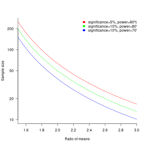
Unless the performance difference between languages is very large (e.g., a factor of three) the required sample size is going to push measurement costs into many tens of millions (£1 million per team, to develop a realistic application, multiplied by two and then multiplied by sample size).
For small programs solving certain kinds of problems, a factor of three, or more, performance difference between languages is not unusual (e.g., me using R for this post, versus using Python). As programs grow, the mundane code becomes more and more dominant, with the special case language performance gains playing an outsized role in story telling.
There have been studies comparing pairs of languages. Unfortunately, most have involved students implementing short problems, one attempted to measure the impact of programming language on coding competition performance (and gets very confused), the largest study I know of compared Fortran and Ada implementations of a satellite ground station support system.
The performance difference detected may be due to the particular problem implemented. The language/problem performance correlation can be solved by implementing a wide range of problems (using 64 teams per language).
A statistically meaningful comparison of the implementation costs of language pairs will take many years and cost many millions. This question is unlikely to every be answered. Move on.
My view is that, at least for the widely used languages, the implementation/maintenance performance issues are primarily driven by the ecosystem, rather than the language.
Optimal function length: an analysis of the cited data
Careful analysis is required to extract reliable conclusions from data. Sloppy analysis can lead to incorrect conclusions being drawn.
The U-shaped plots cited as evidence for an ‘optimal’ number of LOC in a function/method that minimises the number of reported faults in a function, were shown to be caused by a mathematical artifact. What patterns of behavior are present in the data cited as evidence for an optimal number of LOC?
The 2000 paper Module Size Distribution and Defect Density by Malaiya and Denton summarises the data-oriented papers cited as sources on the issue of optimal length of a function/method, in LOC.
Note that the named unit of measurement in these papers is a module. In one paper, a module is specified as being as Ada package, but these papers specify that a module is a single function, method or anything else.
In order of publication year, the papers are:
The 1984 paper Software errors and complexity: an empirical investigation by Basili, and Perricone analyses measurements from a 90K Fortran program. The relevant Faults/LOC data is contained in two tables (VII and IX). Modules are sorted in to one of five bins, based on LOC, and average number of errors per thousand line of code calculated (over all modules, and just those containing at least one error); see table below:
     Module         Errors/1k lines   Errors/1k lines
     max LOC          all modules      error modules
        50              16.0               65.0
       100              12.6               33.3
       150              12.4               24.6
       200               7.6               13.4
>200 6.4 9.7 |
One of the paper’s conclusions: “One surprising result was that module size did not account for error proneness. In fact, it was quite the contrary–the larger the module, the less error-prone it was.”
The 1985 paper Identifying error-prone software—an empirical study by Shen, Yu, Thebaut, and Paulsen analyses defect data from three products (written in Pascal, PL/S, and Assembly; there were three versions of the PL/S product) were analysed using Halstead/McCabe, plus defect density, in an attempt to identify error-prone software.
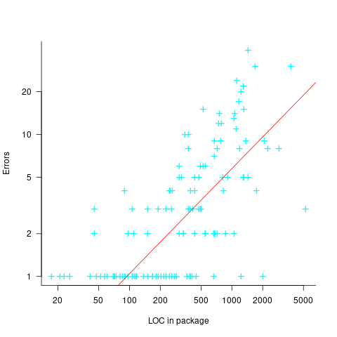
The paper includes a plot (figure 4) of defect density against LOC for one of the PL/S product releases, for 108 modules out of 253 (presumably 145 modules had no reported faults). The plot below shows defects against LOC, the original did not include axis values, and the red line is the fitted regression model  (data extracted using WebPlotDigitizer; code+data):
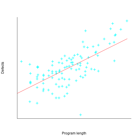
The power-law exponent is less than one, which suggests that defects per line is decreasing as module size increases, i.e., there is no optimal minimum, larger is always better. However, the analysis is incomplete because it does not include modules with zero reported defects.
The authors say: “… that there is a higher mean error rate in smaller sized modules, is consistent with that discovered by Basili and Perricone.”
The 1990 paper Error Density and Size in Ada Software by Carol Withrow analyses error data from a 114 KLOC military communication system written in Ada; of the 362 Ada packages, 137 had at least one error. The unit of measurement is an Ada package, which like a C++ class, can contain multiple definitions of types, variables, and functions.
The paper plots errors per thousand line of code against LOC, for packages containing at least one error, i.e., 62% of packages are not included in the analysis. The 137 packages are sorted into 8-bins, based on the number of lines they contain. The 52 packages in the 159-251 LOC bin have an average of 1.8 errors per 1 KLOC, which is the lowest bin average. The author concludes: “Our study of a large Ada project shows this optimal size to be about 225 lines.”
The plot below shows errors against LOC, red line is the fitted regression model  for
for  (data extracted using WebPlotDigitizer from figure 2; code+data):
The 1993 paper An Empirical Investigation of Software Fault Distribution by Moller, and Paulish analysed four versions of a 750K product for controlling computer system utilization, written in assembler; the items measured were: DLOC (‘delta’ lines of code, DLOC, defined as “… the number of added or modified source lines of code for a version as compared to the prior version.”) and fault rate (faults per DLOC).
This paper is the first to point out that the code from multiple modules may need to be modified to fix a defect/fault/error. The following table shows the percentage of faults whose correction required changes to a given number of modules, for three releases of the product.
                   Modules
   Version  1    2    3     4     5     6
      a    78%  14%  3.4%  1.3%  0.2%  0.1%
      b    77%  18%  3.3%  1.1%  0.3%  0.4%
c 85% 12% 2.0% 0.7% 0.0% 0.0% |
Modules are binned by DLOC and various plots appear in the paper; it’s all rather convoluted. The paper summary says: “With modified code, the fault rates steadily decrease as the module size increases.”
What conclusions does the Malaiya and Denton paper draw from these papers?
They present “… a model giving influence of module size on defect density based on data that has been reported. It provides an interpretation for both declining defect density for smaller modules and gradually rising defect density for larger modules. … If small modules can be
combined into optimal sized modules without reducing cohesion significantly, than the inherent defect density may be significantly reduced.”
The conclusion I draw from these papers is that a sloppy analysis in one paper obtained a result that sounded interesting enough to get published. All the other papers find defect/error/fault rate decreasing with module size (whatever a module might be).
Readability of anonymous inner classes and lambda expressions
The available evidence on readability is virtually non-existent, mostly consisting of a handful of meaningless experiments.
Every now and again somebody runs an experiment comparing the readability of X and Y. All being well, this produces a concrete result that can be published. I think that it would be a much more effective use of resources to run eye tracking experiments to build models of how people read code, but then I’m not on the publish or perish treadmill.
One such experimental comparison of X and Y is the paper Two N-of-1 self-trials on readability differences between anonymous inner classes (AICs) and lambda expressions (LEs) on Java code snippets by Stefan Hanenberg (who ran some experiments on the benefits of strong typing) and Nils Mehlhorn.
How might the readability of X and Y be compared (e.g., Java anonymous inner classes and lambda expressions)?
If the experimenter has the luxury of lots of subjects, then half of the subjects can be assigned to use X and half to use Y. When only a few subjects are available, perhaps as few as one, an N-of-1 experimental design can be used.
This particular study is worth discussing because it appears to be thought out and well run, as well as illustrating the issues involved in running such experiments, not because the readability of the two constructs is of particular interest. I think that developer choice of anonymous inner classes or lambda expressions is based on fashion and/or habit, and developers will claim the construct they use is the most readable one for them.
The Hanenberg and Mehlhorn study involved two experiments, using a N-of-1 design. In the first experiment task, subjects saw a snippet of code and had to count the number of parameters in either the anonymous inner class or the lambda expression (whose parameters were either untyped or typed); in the second experiment task subjects had to count the number of defined parameters that were used in the body of the anonymous inner class or lambda expression. English words were used for parameter names.
Each of the eight subjects saw the same set of randomly shuffled distinct 600 code snippets. The time taken to answer and correct/incorrect answer status were recorded. The snippets varied in the number of parameters and kind of construct; for task 1: 0-4 parameters, 3-kinds of construct, repeated 40 times, giving  distinct snippets; for task 2: 0-3 parameters used out of 3 parameters, 3-kinds of construct, repeated 50 times, giving
  distinct snippets.
The first task requires subjects to locate the definition of the construct, count the number of parameters, and report the count. The obvious model is different constructs require different amounts of time to locate, and that each parameter adds a fixed amount to the response time; there may be a small learning component.
Fitting a simple regression model shows (depending on choice of outlier bounds) that averaged over all subjects each parameter increased response time by around 80 msec, and that response was faster for lambda expressions (around 200 msec without parameter types, 90 msec if types are present); code+data. However, the variation across subjects had a standard deviation that was similar to these means.
The second task required subjects to read the body of the code, to find out which parameters were used. The mean response time increased from 1.5 to 3.7 seconds.
I was not sure whether to expect response time to increase or decrease as the number of parameters used in the body of the code increased (when the actual number of parameters is always three).
A simple fitted regression model finds that increase/decrease behavior varies between subjects (around 50 msec per parameter used); code+data. I am guessing that performance behavior depends on the mental model used to hold the used/not yet used information.
The magnitude of the performance differences found in this study mimics that seen in most human based software engineering experiments, that is, the impact of the studied construct is very small.
Predicting the size of the Linux kernel binary
How big is the binary for the Linux kernel? Depending on the value of around 15,000 configuration options, the size of the version 5.8 binary could be anywhere between 7.3Mb and 2,134 Mb.
Who is interested in the size of the Linux kernel binary?
We are not in the early 1980s, when memory for a desktop microcomputer often topped out at 64K, and software was distributed on 360K floppies (720K when double density arrived; my companies first product was a code optimizer which reduced program size by around 10%).
While desktop systems usually have oodles of memory (disk and RAM), developers targeting embedded systems seek to reduce costs by minimizing storage requirements, security conscious organizations want to minimise the attack surface of the programs they run, and performance critical systems might want a kernel that fits within a processors’ L2/L3 cache.
When management want to maximise the functionality supported by a kernel within given hardware resource constraints, somebody gets the job of building kernels supporting various functionality to find out the size of the binaries.
At around 4+ minutes per kernel build, it’s going to take a lot of time (or cloud costs) to compare lots of options.
The paper Transfer Learning Across Variants and Versions: The Case of Linux Kernel Size by Martin, Acher, Pereira, Lesoil, Jézéquel, and Khelladi describes an attempt to build a predictive model for the size of the kernel binary. This paper includes an extensive list of references.
The author’s approach was to first obtain lots of kernel binary sizes by building lots of kernels using random permutations of on/off options (only on/off options were changed). Seven kernel versions between 4.13 and 5.8 were used, producing 243,323 size/option setting combinations (complete dataset). This data was used to train a machine learning model.
The accuracy of the predictions made by models trained on a single kernel version were accurate within that kernel version, but the accuracy of single version trained models dropped dramatically when used to predict the binary size of later kernel versions, e.g., a model trained on 4.13 had an accuracy of 5% MAPE predicting 4.13, when predicting 4.15 the accuracy is 20%, and 32% accurate predicting 5.7.
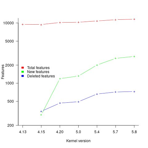
I think that the authors’ attempt to use this data to build a model that is accurate across versions is doomed to failure. The rate of change of kernel features (whose conditional compilation is supported by one or more build options) supported by Linux is too high to be accurately modelled based purely on information of past binary sizes/options. The plot below shows the total number of features, newly added, and deleted features in the modelled version of the kernel (code+data):
What is the range of impacts of each build option, on binary size?
If each build option is independent of the others (around 44% of conditional compilation directives in the kernel source contain one option), then the fitted coefficients of a simple regression model gives the build size increment when the corresponding option is enabled. After several cpu hours, the 92,562 builds involving 9,469 options in the version 4.13 build data were fitted. The plot below shows a sorted list of the size contribution of each option; the model  is 0.72, i.e., quite a good fit (code+data):

While the mean size increment for an enabled option is 75K, around 40% of enabled options decreases the size of the kernel binary. Modelling pairs of options (around 38% of conditional compilation directives in the kernel source contain two options) will have some impact on the pattern of behavior seen in the plot, but given the quality of the current model ( is 0.72) the change is unlikely to be dramatic. However, the simplistic approach of regression fitting the 90 million pairs of option interactions is not practical.
What might be a practical way of estimating binary size for any kernel version?
The size of a binary is essentially the quantity of code+static data it contains.
An estimate of the quantity of conditionally compiled source code dependent on a given option is likely to be a good proxy for that option’s incremental impact on binary size.
It’s trivial to scan source code for occurrences of options in conditional compilation directives, and with a bit more work, the number of lines controlled by the directive can be counted.
There has been a lot of evidence-based research on software product lines, and feature macros in particular. I was expecting to find a dataset listing the amount of code controlled by build options in Linux, but the data I can find does not measure Linux.
The Martin et al. build data is perfectfor creating a model linking quantity of conditionally compiled source code to change of binary size.
Perturbed expressions may ‘recover’
This week I have been investigating the impact of perturbing the evaluation of random floating-point expressions. In particular, the impact of adding 1 (and larger values) at a random point in an expression containing many binary operators (simply some combination of add/multiply).
What mechanisms make it possible for the evaluation of an expression to be unchanged by a perturbation of +1.0 (and much larger values)? There are two possible mechanisms:
- the evaluated value at the perturbation point is ‘watered down’ by subsequent operations, such that the original perturbed value makes no contribution to the final result. For instance, the IEEE single precision float mantissa is capable of representing 6-significant digits; starting with, say, the value
0.23, perturbing by adding1.0gives1.23, followed by a sequence of many multiplications by values between zero and one could produce, say, the value6.7e-8, which when added to, say,0.45, gives0.45, i.e., the perturbed value is too small to affect the result of the add, - the perturbed branch of the expression evaluation is eventually multiplied by zero (either because the evaluation of the other branch produces zero, or the operand happens to be zero). The exponent of an IEEE single precision float can represent values as small as
1e-38, before underflowing to zero (ignoring subnormals); something that is likely to require many more multiplies than required to lose 6-significant digits.
The impact of a perturbation disappears when its value is involved in a sufficiently long sequence of repeated multiplications.
The probability that the evaluation of a sequence of  multiplications of random values uniformly distributed between zero and one produces a result less than is given by
 }/{(N-1)!}") , where
, where  is the incomplete gamma function, and
  is the upper bounds (1 in our case). The plot below shows this cumulative distribution function for various (code):
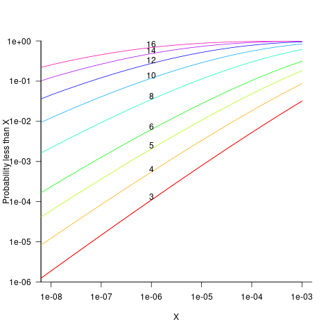
Looking at this plot, a sequence of 10 multiplications has around a 1-in-10 chance of evaluating to a value less than 1e-6.
In practice, the presence of add operations will increase the range of operands values to be greater than one. The expected distribution of result values for expressions containing various percentages of add/multiply operators is covered in an earlier post.
The probability that the evaluation of an expression involves a sequence of multiplications depends on the percentage of multiply operators it contains, and the shape of the expression tree. The average number of binary operator evaluations in a path from leaf to root node in a randomly generated tree of operands is proportional to  .
.
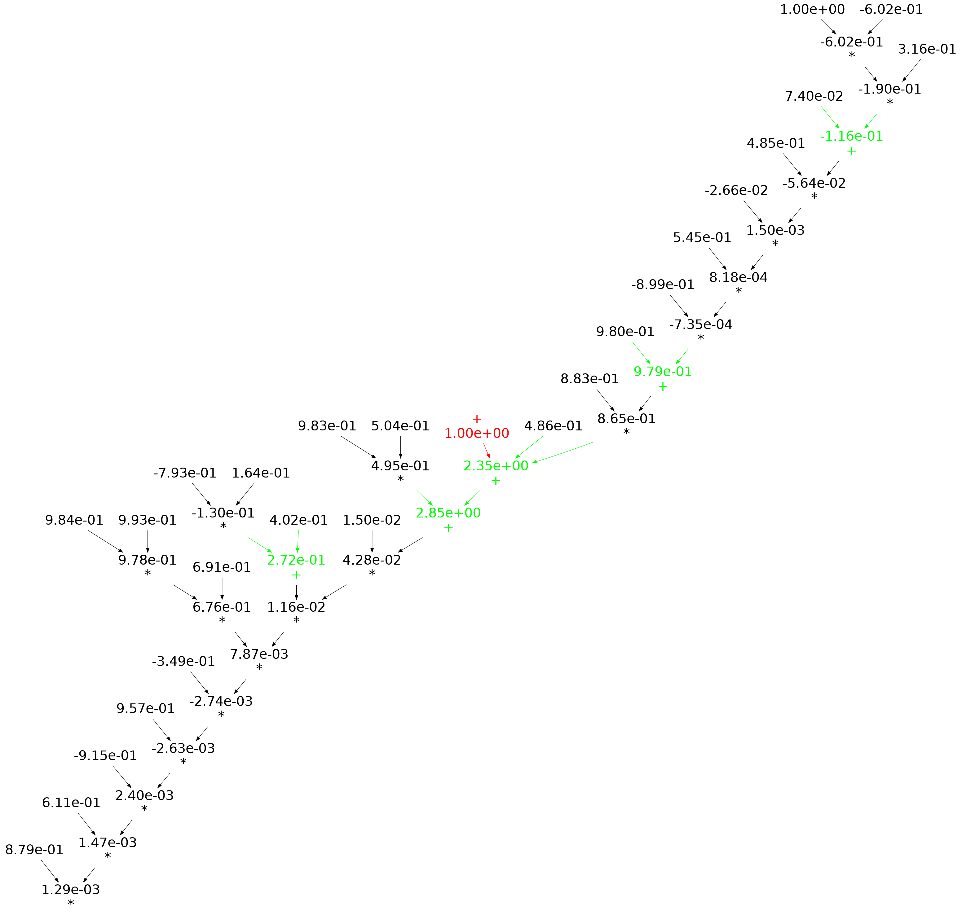
When an expression has a ‘bushy’ balanced form, there are many relatively distinct evaluation paths, the expected number of operations along a path is proportional to  . The plot below shows a randomly generated ‘bushy’ expression tree containing 25 binary operators, with 80% multiply, and randomly selected values (perturbation in red, additions in green; code+data):
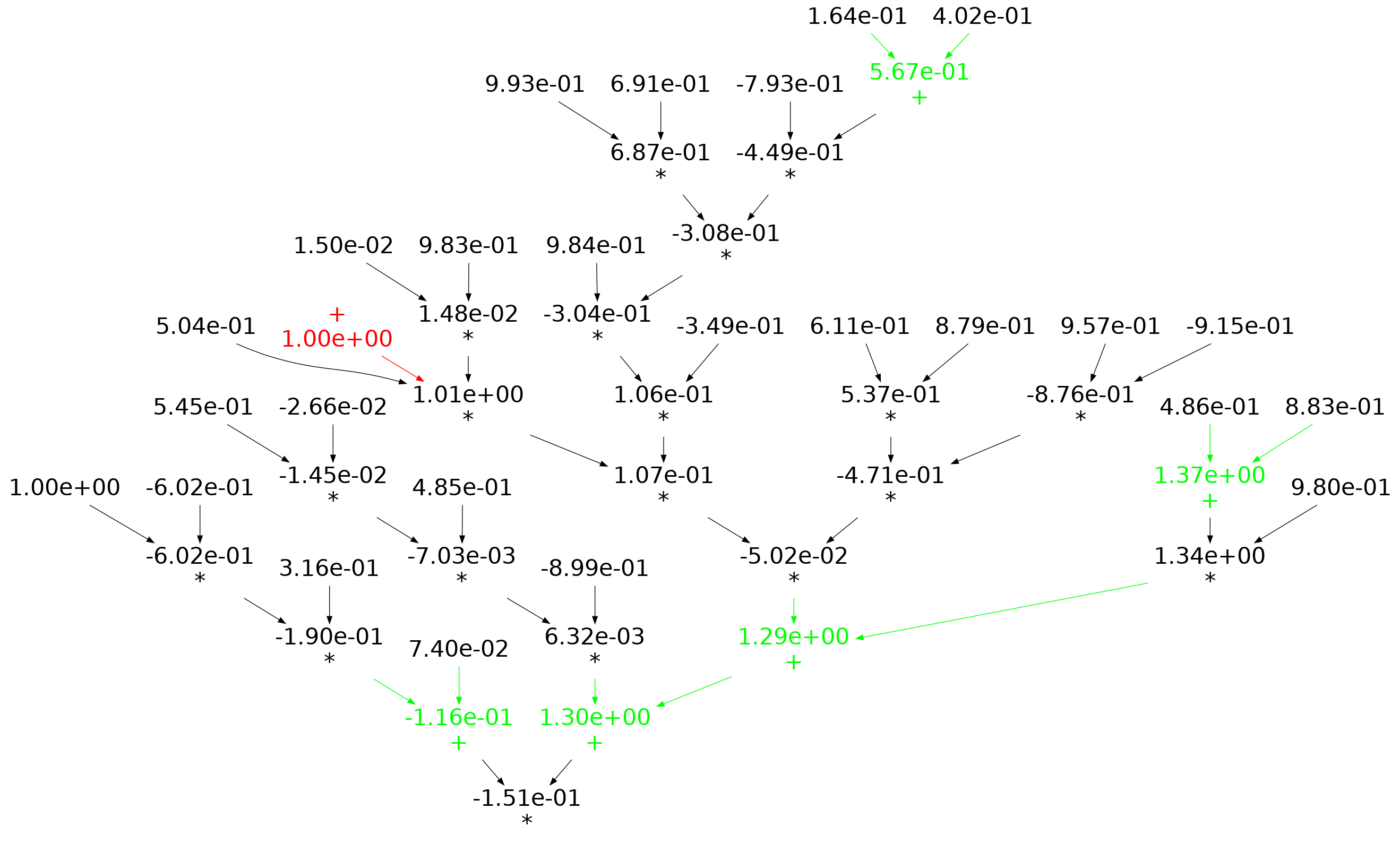
When an expression has a ‘tall’ form, there is one long evaluation path, with a few short paths hanging off it, the expected number of operations along the long path is proportional to . The plot below shows a randomly generated ‘tall’ expression tree containing 25 binary operators, with 80% multiply, and randomly selected values (perturbation in red, additions in green; code+data):
If, one by one, the result of every operator in an expression is systematically perturbed (by adding some value to it), it is known that in some cases the value of the perturbed expression is the same as the original.
The following results were obtained by generating 200 random C expressions containing some percentage of add/multiply, some number of operands (i.e., 25, 50, 75, 100, 150), one-by-one perturbing every operator in every expression, and comparing the perturbed result value to the original value. This process was repeated 200 times, each time randomly selecting operand values from a uniform distribution between -1 and 1. The perturbation values used were: 1e0, 1e2, 1e4, 1e8, 1e16. A 32-bit float type was used throughout.
Depending on the shape of the expression tree, with 80% multiplications and 100 operands, the fraction of perturbed expressions returning an unchanged value can vary from 1% to 40%.
The regression model fitted to the fraction of unchanged expressions contains lots of interactions (the simple version is that the fraction unchanged increases with more multiplications, decreases as the log of the perturbation value, the square root of the number of operands is involved; code+data):
*(sqrt{OPD}-0.007*AM)+sqrt{OPD}(0.05-0.08*AM)")
where:  is the fraction of perturbed expressions returning the original value,
  the percentage of add operators (not multiply),
  the number of operands in the expression, and
  the perturbation value.
There is a strong interaction with the shape of the expression tree, but I have not found a way of integrating this into the model.
The following plot shows the fraction of expressions unchanged by adding one, as the perturbation point moves up a tall tree, x-axis, for expressions containing 50 and 100 operands, and various percentages of multiplications (code+data):
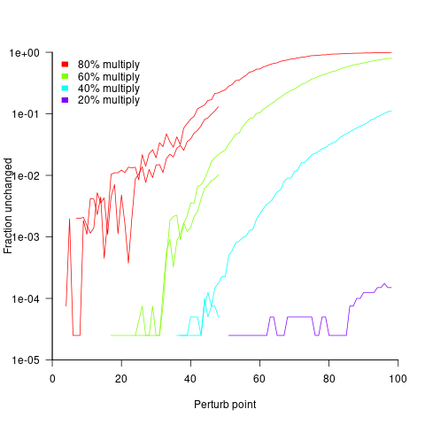
No attempt was made to count the number of expression evaluations where the perturbed value was eventually multiplied by zero (the second bullet point discussed at the start).
Human reasoning is generally not logic based
From around 350 BC until the 1960s, the students were taught that people reasoned using logic, and teachers believed this to be true. In the 1960s psychologists started running experiments that asked subjects to solve reasoning problems, the results showed that people often failed to give the answers dictated by logic.
Some recurring patterns were present in the answers given, and small changes in the wording of the question asked were found to produce different answer patterns. Very few researchers were willing to give up the idea that subjects were reasoning using logic, there must be another explanation, e.g., subjects must be interpreting the experimental questions asked in a way that differed from that assumed by the researchers. The social context of reasoning was one of the early drivers of evolutionary psychology; reasoning must provide some survival benefit by solving problems that regularly occur in natural human environments.
After a myriad of detailed theories did little more than predict small subsets of subject responses, mainstream reasoning research finally gave up the belief that logic is the default technique used by people to solve reasoning problems. Theories of reasoning behavior are now based around people estimating probabilities and picking the answer with the highest probability; this approach does a much better job of predicting common patterns in subject answers.
Experimental studies of reasoning often use psychology undergraduates as subjects (the historical norm, with Mechanical Turk workers becoming more common). While researchers may be concerned about how well undergraduate behavior mimics the general population, my concern is the extent to which these results apply to software developers. Is a necessary condition for being a professional software developer that a person, by default, uses logic to solve reasoning problems?
Of course, software developers claim that their reasoning is logic based, but then so do people in the general population (or at least the non-developers I interact with do). The dual-process theory of reasoning contains two reasoning systems, one unconscious/intuitive and the second a conscious/deliberate system; it has been said that the purpose of the second system is to come up with reasons to justify the answers produced by the first system.
Until reasoning experiments are run with professional developer subjects, we won’t know the extent to which existing results in reasoning research apply to this specialist subset of the population.
The Wason selection task is to studies of reasoning, like the fruit fly is to studies of genetics. What pattern of behavior do you show on this task (code)?
The plot below shows a set of four cards, of which you can see only the exposed face but not the hidden back. On each card, there is a number on one side and a letter on the other.
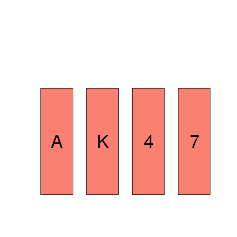
- Given the statement: “If there is a vowel on one side, then there is an even number on the other side.”
Your task is to decide, which, if any, of these four cards must be turned over to decide whether this statement is true. - Specify the cards you would turn over. Don’t turn unnecessary cards.
————————————
Most people correct specify that the card showing a vowel must be turned over to verify that an even number appears on the other side. A common mistake is to specify that the card showing an even number also has to be turned over. However, there is no requirement on the letter appearing on the other side of a card showing an even number. A second necessary condition involves a negative test (something that developers are known to overlook); for the statement to hold, a vowel must not appear on the other side of the card showing an odd number, this is the second card that must be turned over.
Recent Comments