Archive
Modelling estimate/actual including uncertainty in the estimate
What is an effective technique for modelling the relationship between the time estimated to implement a task and the actual time taken to implement that task?
A regression model is the obvious approach. However, an important assumption made by the commonly used regression techniques is not met by estimate/actual project data
The commonly used regression techniques involve two kinds of variables: the explanatory variable and the response variable (also known as the independent and dependent variables). For instance, in the equation  ,
,  is the explanatory variable and
  is the response variable.
When fitting a regression model to measurement data, the fitted equation is assumed to have the form such as:  , where
  is uncertainty in the value of , with the valued assumed to have no uncertainty;
  and
and  are constants fitted by the modelling process. The values returned by the model fitting process include an estimate for , as well as estimates for and .
When running an experiment, the values of the explanatory variables(e.g., ) are chosen by the experimenter, with the subject providing the value of the response variable, e.g., .
What does this technical detail have to do with estimation data?
The task estimate/actual values are both provide by the subject (i.e., the developer), there is no experimenter providing one of the values; in fact there is no experiment, these are measurements of things that happened. Both the estimate and actual are response variables, and both contain some amount of uncertainty, and the fitting process needs to take this into account. The appropriate regression technique to use for this case is an errors-in-variables model, which fits the equation +epsilon") , with
, with  being the uncertainty in .
A previous post discussed the surprising behavior that can occur when failing to use errors-in-variables regression for where the data does not contain any explanatory variables, i.e., all the variables contain uncertainty.
The process of fitting an errors-in-variables regression model requires additional input, a value for has to be specified. Taking the example of task estimation, possible uncertainties in the estimate include: misunderstanding of the requirement(s), faded memory of the actual time previously taken by very similar tasks, an inaccurate model of developer skills, and a preference for using round numbers.
What data is available on the uncertainty of individual task estimates? I know of one study where, unknown to them, the individuals estimated the same task twice (in fact, seven people each estimated the same six distinct tasks twice, over a period of three-months). The plot below shows the first/second estimate made by each person for each of the six tasks, with the grey line showing where first==second estimate (code+data):
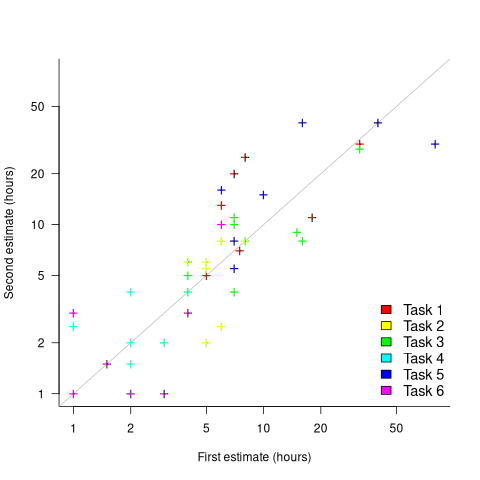
Assuming the estimation uncertainty in this experiment’s data is roughly equal to the estimation uncertainty in other estimation datasets, of tasks taking up to 20 hours, how might it be used to calculate a value for the uncertainty in estimated values?
Two possibilities include:
- Assuming that the uncertainty in both the first and second estimates is equal, a model can be fitted using Deming regression (which treats both variables as having the same uncertainty), and the residual standard error of this model used as the value of . This value for a fitted multiplicative model is 0.6 (code+data),
- using the mean of the relative errors,
}/Est_1") ; its value is 0.55.
; its value is 0.55.
How different are the models built using linear regression and errors-in-variables regression, for small task estimates?
A basic linear regression model fitted to the SiP estimation dataset is:  .
.
Updating this model, using SIMEX, to take into uncertainty in the value of  gives, for an uncertainty error of 0.55:
  , and for an uncertainty error of 0.60:
  . The coefficients for the two models are essentially the same (code+data).
The exponent value is the noticeable difference between the linear regression and errors-in-variables regression models. Adding the assumed amount of uncertainty (based on data from one experiment) to the estimated value leads to a model where estimate/actual are very close to having a linear relationship.
Is this errors-in-variables model any closer to reality than the linear regression model? The model shows that the estimate/actual relationship is closer to linear than was previously thought. Until more data becomes available, we won’t know how close this relationship actually is.
The people who made the estimates in the SiP data also performed the work that took the recorded actual time. Assigning a task to a different person could produce both a different estimate and a different actual, but these possible values are unknown. On a larger scale, different companies bidding on the same contract specify different amounts and have different implementations times; data showing these differences.
Percolation of the impact of coding mistakes through a program
Programs containing serious coding mistakes can sometimes work surprisingly well. Experienced developers invariably have a story to tell about a program in production use that contained a coding mistake so bad, that it should have prevented the program producing any reliably output. My story relates to a Z80 cpu emulator I had written, which was successfully booting/running CP/M and several applications. One application was sometimes behaving erratically. I eventually traced the problem to the implementation of one of the add instructions (there are 13 special cases), which had been cut/pasted from the implementation of the corresponding subtract instruction, except that I had forgotten to change the result calculation from using a subtract to using an add, i.e., the instruction was performing a subtract, not an add. I was flabbergasted that so much emulated code appeared to be working in the presence of what to me was a crippling coding mistake.
There have been a handful of studies investigating the ability of programs containing coding mistakes to function correctly, or at least well enough to be usable.
- The earliest paper I have found is from 2005; Rinard, Cadar and Nguyen changed the termination condition of 326
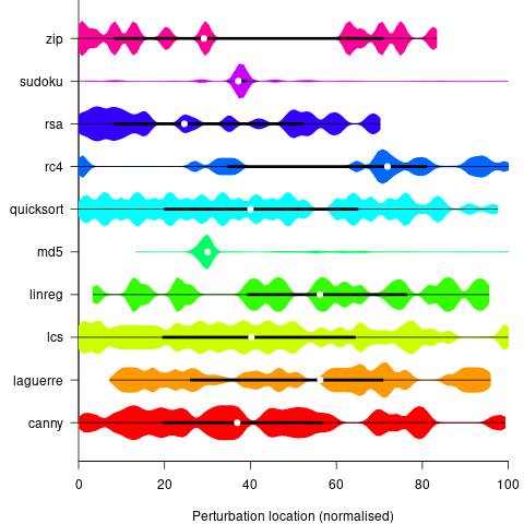
for-loopsin the Pine email client, with<becoming<=, and>becoming>=. While the resulting program exhibited obvious anomalies, the researchers were able to use it to send and receive email, - a study by Danglot, Preux, Baudry and Monperrus investigated the propagation of single perturbations in 10 short Java programs (42 to 568 LOC, perturbed by adding/subtracting 1 from an expression somewhere in the code). The plot below shows the likelihood that a perturbation at some point in the code will have no impact on the output; code+data,
- a study by Cho of the impact of soft errors (i.e., radiation induced bit-flips) found that over 80% of bit-flips had no detectable impact on program behavior.
This week I attended the 63rd CREST Open Workshop; the topic was genetic improvement of software, i.e., GI randomly combines members of a population of programs, only keeping the children that pass some fitness test, rinses and repeats until one or more programs reach some acceptance threshold.
The GI community recently discovered that program output is often unaffected by a small perturbation to program execution, e.g., randomly adding one to the result of a binary operation.
A study by Langdon, Al-Subaihin and Clark tracked the effect of perturbations in the evaluation of an expression tree. The expression trees were created using genetic programming, with the fitness function being the difference between the value obtained by evaluating the expression tree and a sixth order polynomial. The binary operators in the expression tree were multiply and addition, with the leaf node value, x, taking a value between -0.97789 and 0.979541; the trees were a lot deeper than the one below, containing between 8.9k and 863k nodes/leafs, with tree depth varying from 121 to 5,103.
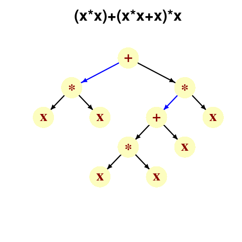
During the evaluation of an expression tree the result of one of the multiply/add operations was perturbed by adding one to its value. The subsequent evaluation of the remainder of the expression tree was tracked, comparing original/perturbed calculated values until either the root node was reached (and the final result was different), or the original/perturbed subtree result values synchronized, i.e., became the same. The distance, in nodes, between perturbation and value synchronization was recorded.
In all, ten expression trees were created, and each node in every tree was perturbed once per run; there were 10 runs using 10 different values of x.
The plot below shows results from two expression trees (different colors). Each point is the distance before original/perturbed values synchronised (for those cases where this happened) against the number of runs having this distance (for the same tree; code+data, and thanks to Bill for explaining things):
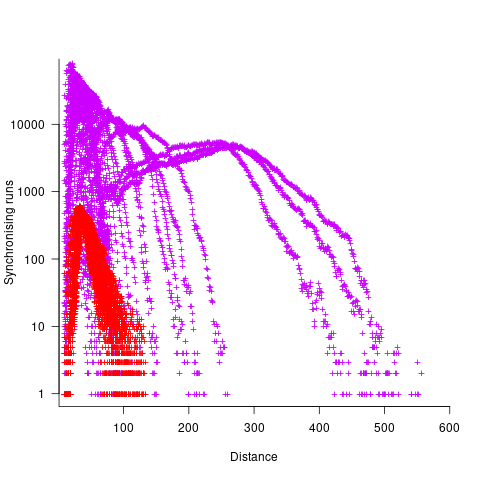
For the larger tree, there is a distinct pattern for each of the ten input values, x. This shows that synchronisation distance can be affected by the input value (which is to be expected). Perhaps this pattern is not present in the smaller tree, or the points are too close together to see it.
The opportunities available to a perturbation for travelling some distance depends on the size and characteristics of the expression tree, with a large thin tree providing more opportunities for longer distance travel than a large bushy tree.
It will take some well thought through experiments to unpick the contributions made by the tree characteristics, problem characteristics, and the prevalence of binary operators unlikely to be affected by small changes to their operand value, e.g., there is roughly a 50% chance that a relational comparison will be unaffected by a small change to one of its operands.
If you know of any other studies investigating coding mistake percolation, please let me know.
Evaluating Story point estimation error
If a task implementation estimate is expressed in time, various formula are available for evaluating how well the estimated time corresponds to the actual time.
When an estimate is expressed in story points, how might the estimate be evaluated when actual time is measured in hours?
The common practice of selecting story point values from a small set of integers (I have seen fractional values used) introduces quantization error into most estimates (around 30% of time estimates equal actual time), assuming that actual times are not constrained to a similar number of possible time values.
If we assume a linear mapping from estimated story points to actual time and an ideal estimator (let’s assume that 1 story point is equivalent to 1 hour), then a lower bound on the error can be calculated.
Our ideal estimator is able to exactly predict the actual time. However, the use of story points means that this exact prediction has to be rounded to one of a small set of integer values. Let’s assume that our ideal estimator rounds to the story point value that is closest to the exact prediction, e.g., all story points predicted to take up to 1.5 are estimated at 1 story point.
What is the mean error of the estimates made by this ideal, rounded, estimator?
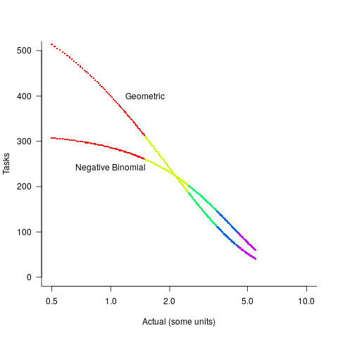
The available evidence shows that the distribution of tasks having a given actual implementation time roughly has the form of a geometric (the discrete form of exponential) or negative binomial distribution. The plot below shows a geometric and negative binomial distribution, with distinct colors over the range where values are rounded to the same closest integer (dots are at 1-minute intervals, code):
Having picked a distribution for actual times, we can calculate the number of tasks estimated to require, for instance, 1 story point, but actually taking 1 hour, 1 hr 1 min, 1 hr 2 min, …, 1 hr 30 min. The mean error can be calculated over each pair of estimate/actual, for one to five story points (in this example). The table below lists the mean error for two actual distributions, calculated using four common metrics: squared error (SE), absolute error (AE), absolute percentage error (APE), and relative error (RE); code:
Distribution SE AE APE RE Geometric 0.087 0.26 0.17 0.20 Negative Binomial 0.086 0.25 0.14 0.16 |
A few minutes difference in a 1 SP estimate is a larger error than the same number of minutes in a two or more SP estimate, combined with most tasks take a small amount of time, means that error estimation is dominated by inaccuracies in estimating small tasks.
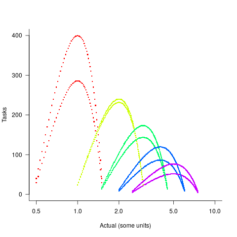
In practice, the range of actual times, for a given estimate, is better approximated by a percentage of the estimated time (50% is used below), and the number of tasks having a given actual value for a given estimate, approximated by a triangular distribution (a cubic equation was used for the following calculation). The plot below shows the distribution of estimation points around a given number of story points (at 1-minute intervals), and the geometric and negative binomial distribution (compare against plot above to work out which is which; code):
The following table lists of mean errors:
Distribution SE AE APE RE Geometric 0.52 0.55 0.13 0.13 Negative Binomial 0.62 0.61 0.13 0.14 |
When the error in the actual is a percentage of the estimate, larger estimates have a much larger impact on absolute accuracy; see the much larger SE and AE values. The impact on the relative accuracy metrics appears to be small.
Is evaluating estimation error useful, when estimates are given in story points?
While it’s possible to argue for and against, the answer is that usefulness is in the eye of the beholder. If development teams find the information useful, then it is useful; otherwise not.
Evaluating estimation performance
What is the best way to evaluate the accuracy of an estimation technique, given that the actual values are known?
Estimates are often given as point values, and accuracy scoring functions (for a sequence of estimates) have the form }") , where
, where  is the number of estimated values,
  the estimates, and
  the actual values; smaller
  is better.
Commonly used scoring functions include:
=(E-A)^2") , known as squared error (SE)
, known as squared error (SE)=delim{|}{E-A}{|}") , known as absolute error (AE)
, known as absolute error (AE)=delim{|}{E-A}{|}/A") , known as absolute percentage error (APE)
, known as absolute percentage error (APE)=delim{|}{E-A}{|}/E") , known as relative error (RE)
, known as relative error (RE)
APE and RE are special cases of: =delim{|}{1-(A/E)^{beta}}{|}") , with
, with  and
and  respectively.
Let’s compare three techniques for estimating the time needed to implement some tasks, using these four functions.
Assume that the mean time taken to implement previous project tasks is known,  . When asked to implement a new task, an optimist might estimate 20% lower than the mean,
  , while a pessimist might estimate 20% higher than the mean,
  . Data shows that the distribution of the number of tasks taking a given amount of time to implement is skewed, looking something like one of the lines in the plot below (code):
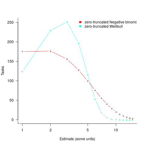
We can simulate task implementation time by randomly drawing values from a distribution having this shape, e.g., zero-truncated Negative binomial or zero-truncated Weibull. The values of  and
and  are calculated from the mean, , of the distribution used (see code for details). Below is each estimator’s score for each of the scoring functions (the best performing estimator for each scoring function in bold; 10,000 values were used to reduce small sample effects):
    SE   AE   APE   RE

  2.73 1.29 0.51 0.56

 2.31 1.23 0.39 0.68

  2.70 1.37 0.36 0.86
Surprisingly, the identity of the best performing estimator (i.e., optimist, mean, or pessimist) depends on the scoring function used. What is going on?
The analysis of scoring functions is very new. A 2010 paper by Gneiting showed that it does not make sense to select the scoring function after the estimates have been made (he uses the term forecasts). The scoring function needs to be known in advance, to allow an estimator to tune their responses to minimise the value that will be calculated to evaluate performance.
The mathematics involves Bregman functions (new to me), which provide a measure of distance between two points, where the points are interpreted as probability distributions.
Which, if any, of these scoring functions should be used to evaluate the accuracy of software estimates?
In software estimation, perhaps the two most commonly used scoring functions are APE and RE. If management selects one or the other as the scoring function to rate developer estimation performance, what estimation technique should employees use to deliver the best performance?
Assuming that information is available on the actual time taken to implement previous project tasks, then we can work out the distribution of actual times. Assuming this distribution does not change, we can calculate APE and RE for various estimation techniques; picking the technique that produces the lowest score.
Let’s assume that the distribution of actual times is zero-truncated Negative binomial in one project and zero-truncated Weibull in another (purely for convenience of analysis, reality is likely to be more complicated). Management has chosen either APE or RE as the scoring function, and it is now up to team members to decide the estimation technique they are going to use, with the aim of optimising their estimation performance evaluation.
A developer seeking to minimise the effort invested in estimating could specify the same value for every estimate. Knowing the scoring function (top row) and the distribution of actual implementation times (first column), the minimum effort developer would always give the estimate that is a multiple of the known mean actual times using the multiplier value listed:
                   APE   RE

Negative binomial  1.4   0.5

Weibull            1.2   0.6
For instance, management specifies APE, and previous task/actuals has a Weibull distribution, then always estimate the value  .
.
What mean multiplier should Esta Pert, an expert estimator aim for? Esta’s estimates can be modelled by the equation ") , i.e., the actual implementation time multiplied by a random value uniformly distributed between 0.5 and 2.0, i.e., Esta is an unbiased estimator. Esta’s table of multipliers is:
, i.e., the actual implementation time multiplied by a random value uniformly distributed between 0.5 and 2.0, i.e., Esta is an unbiased estimator. Esta’s table of multipliers is:
                   APE     RE

Negative binomial  1.0   0.7

Weibull                     1.0     0.7
A company wanting to win contracts by underbidding the competition could evaluate Esta’s performance using the RE scoring function (to motivate her to estimate low), or they could use APE and multiply her answers by some fraction.
In many cases, developers are biased estimators, i.e., individuals consistently either under or over estimate. How does an implicit bias (i.e., something a person does unconsciously) change the multiplier they should consciously aim for (having analysed their own performance to learn their personal percentage bias)?
The following table shows the impact of particular under and over estimate factors on multipliers:
                 0.8 underestimate bias   1.2 overestimate bias

Score function          APE   RE            APE   RE

Negative binomial        1.3   0.9           0.8   0.6

Weibull                 1.3       0.9           0.8   0.6
Let’s say that one-third of those on a team underestimate, one-third overestimate, and the rest show no bias. What scoring function should a company use to motivate the best overall team performance?
The following table shows that neither of the scoring functions motivate team members to aim for the actual value when the distribution is Negative binomial:
                    APE      RE

Negative binomial    1.1     0.7

Weibull                               1.0       0.7
One solution is to create a bespoke scoring function for this case. Both APE and RE are special cases of a more general scoring function (see top). Setting  in this general form creates a scoring function that produces a multiplication factor of 1 for the Negative binomial case.
Initial impressions of RangeLab
I was rummaging around in the source of R looking for trouble, as one does, when I came across what I believed to be a less than optimally accurate floating-point algorithm (function R_pos_di in src/main/arithemtic.c). Analyzing the accuracy of floating-point code is notoriously difficult and those having the required skills tend to concentrate their efforts on what are considered to be important questions. I recently discovered RangeLab, a tool that seemed to be offering painless floating-point code accuracy analysis; here was an opportunity to try it out.
Installation went as smoothly as newly released personal tools usually do (i.e., some minor manual editing of Makefiles and a couple of tweaks to the source to comment out function calls causing link errors {mpfr_random and mpfr_random2}).
RangeLab works by analyzing the flow of values through a program to produce the set of output values and the error bounds on those values. Input values can be specified as a range, e.g., f = [1.0, 10.0] says f can contain any value between 1.0 and 10.0.
My first RangeLab program mimicked the behavior of the existing code in R_pos_di:
n=-10; f=[1.0, 10.0]; res = 1.0; if n < 0, n = -n; f = 1 / f; end while n ~= 0, if (n / 2)*2 ~= n, res = res * f; end n = n / 2; if n ~= 0, f = f*f; end end |
and told me that the possible range of values of res was:
res ans = float64: [1.000000000000001E-10,1.000000000000000E0] error: [-2.109423746787798E-15,2.109423746787799E-15] |
Changing the code to perform the divide last, rather than first, when the exponent is negative:
n=-10; f=[1.0, 10.0]; res = 1.0; is_neg = 0; if n < 0, n = -n; is_neg = 1 end while n ~= 0, if (n / 2)*2 ~= n, res = res * f end n = n / 2; if n ~= 0, f = f*f end if is_neg == 1, res = 1 / res end end |
and the error in res is now:
res ans = float64: [1.000000000000000E-10,1.000000000000000E0] error: [-1.110223024625156E-16,1.110223024625157E-16] |
Yea! My hunch was correct, moving the divide from first to last reduces the error in the result. I have reported this code as a bug in R and wait to see what the R team think.
Was the analysis really that painless? The Rangelab language is somewhat quirky for no obvious reason (e.g., why use ~= when everybody uses != these days and if conditionals must be followed by a character why not use the colon like Python does?) It would be real useful to be able to cut and paste C/C++/etc and only have to make minor changes.
I get the impression that all the effort went into getting the analysis correct and user interface stuff was a very distant second. This is the right approach to take on a research project. For some software to make the leap from interesting research idea to useful tool it is important to pay some attention to the user interface.
The current release does not deserve to be called 1.0 and unless you have an urgent need I would suggest waiting until the usability has been improved (e.g., error messages give some hint about what is wrong and a rough indication of which line the problem occurs on).
RangeLab has shown that there is simpler method of performing useful floating-point error analysis. With some usability improvements RangeLab would be an essential tool for any developer writing code involving floating-point types.
Update: The R team, in the form of Martin Maechler, resolved my report in just over 14 hours! The function R_pos_di is not called, the pow function from the C library (which takes two double arguments rather than a double and an int) has been found to be more accurate. Martin says this usage is not less accurate even for n=3, which I find surprising; I agree it should be more accurate for large values of n.
pow is one of the more complicated maths functions, involving finding a log, a multiply and then returning the exponent of this result. There are lots of boundary values that need to be checked and the code goes on for a while. I will wait for the usability of RangeLab to improve before attempting to compare its accuracy against the simpler algorithm for integer powers. Looking at the SunOracle library sources, if both arguments have integral values the ‘integer power’ algorithm is used (with the divide performed last).
Recent Comments