Archive
Distribution of method chains in Java and Python
Some languages support three different ways of organizing a sequence of functions/methods, with calls taking as their first argument the value returned by the immediately prior call. For instance, Java supports the following possibilities:
r1=f1(val); r2=f2(r1); r3=f3(r2); // Sequential calls r3=f3(f2(f1(val))); // Nested calls, read right to left r3=val.f1().f2().f3(); // Method chain, read left to right |
Simula 67 was the first language to support the dot-call syntax used to code method chains. Ten years later Smalltalk-76 supported sending a message to the result of a prior send, which could be seen as a method chain rather than a nested call (because it is read left to right; Smalltalk makes minimal use of punctuator characters, so the syntax is not distinguishable).
How common are method chains in source code, and what is the distribution of chain length? Two studies have investigated this question: An Empirical Study of Method Chaining in Java by Nakamaru (PhD thesis), Matsunaga, Akiyama, Yamazaki, and Chiba, and Method Chaining Redux: An Empirical Study of Method Chaining in Java, Kotlin, and Python by Keshk, and Dyer.
The plot below shows the number of Java method chains having a given length, for code available in a given year. The red line is a fitted regression line for 2018, based on a model fitted to the complete dataset (code and data):
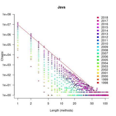
The fitted regression model is:

Why is the number of chains of all lengths growing by around 46% per year? I think this growth is driven by the growth in the amount of source measured. Measurements show that the percentage of source lines containing a method call is roughly constant. In the plot above, the number of unchained methods (i.e., chains of length one) increases in-step with the growth of chained methods. All chain lengths will grow at the same rate, if the source that contains them is growing.
What is responsible for the step change in the number of chains at around 10 methods? Nakamaru classified a random sample of 280 chains, and found that roughly 80% of chains longer than eight methods built an object, e.g., the following chain:
MoreObjects.toStringHelper(this) .add("iLine" , iLine) .add("lastK" , lastK) .add("spacesPending", spacesPending) .add("newlinesPending", newlinesPending) .add("blankLines", blankLines) .add("super", super.toString()) .toString() |
Are these chain usage patterns present in Python? The plot below shows the number of Python method chains having a given length, for code available in a given year. The red line is a fitted regression line for 2020, based on a model fitted to the complete dataset (code and data):

The fitted regression model is:

While this model is almost identical to the model fitted to the Java data (the annual growth rate is 39%), the above plot shows a large step change after chains of length two. Keshk’s paper focuses on replicating Nakamaru’s Java results, and then briefly discusses Python. I have an assortment of explanations, but nothing stands out.
Within code, how are method calls split between single calls and a chain of two or more calls?
The fractions in the plot below are calculated as the ratio of chains of length one (i.e., single method call) against chains containing two or more methods. The “j” shows Java ratios, and “p” Python ratios. The red lines show the fraction based on the total number of method calls, and the blue/green lines are based on occurrences of chains, i.e., chain of one vs chain of many (code and data):

The ratio of Java chains containing two or more methods vs one method, grew by around 6% a year between 2006 and 2018, which is only a small part of the overall 46% annual Java growth.
Method chaining is three times more common in Java than Python. In 2020 around a quarter of all method calls were in a chain of two or more, and single method calls were around ten times more common than multi-call chains.
In Python, the use of method chains has roughly remained unchanged over 15 years, with around 5% of all method calls appearing in a chain.
I don’t have a good idea for why method chains are three times more common in Java than Python. Are nested calls the more common usage in Python, or do developers use a sequence of calls communicating using temporary variables?
What of languages that don’t support method chaining, e.g., C. Is the distribution of the number of nested calls (or sequence of calls using temporaries) a power law with an exponent close to 3.7?
Suggestions and pointers to more data welcome.
Distribution of add/multiply expression values
The implementation of scientific/engineering applications requires evaluating many expressions, and can involve billions of adds and multiplies (divides tend to be much less common).
Input values percolate through an application, as it is executed. What impact does the form of the expressions evaluated have on the shape of the output distribution; in particular: What is the distribution of the result of an expression involving many adds and multiplies?
The number of possible combinations of add/multiply grows rapidly with the number of operands (faster than the rate of growth of the Catalan numbers). For instance, given the four interchangeable variables: w, x, y, z, the following distinct expressions are possible: w+x+y+z, w*x+y+z, w*(x+y)+z, w*(x+y+z), w*x*y+z, w*x*(y+z), w*x*y*z, and w*x+y*z.
Obtaining an analytic solution seems very impractical. Perhaps it’s possible to obtain a good enough idea of the form of the distribution by sampling a subset of calculations, i.e., the output from plugging random values into a large enough sample of possible expressions.
What is needed is a method for generating random expressions containing a given number of operands, along with a random selection of add/multiply binary operators, then to evaluate these expressions with random values assigned to each operand.
The approach I used was to generate C code, and compile it, along with the support code needed for plugging in operand values (code+data).
A simple method of generating postfix expressions is to first generate operations for a stack machine, followed by mapping this to infix form to a postfix form.
The following awk generates code of the form (‘executing’ binary operators, o, right to left): o v o v v. The number of variables in an expression, and number of lines to generate, are given on the command line:
# Build right to left function addvar() { num_vars++ cur_vars++ expr="v " expr # choose variable later } function addoperator() { cur_vars-- expr="o " expr # choose operator later } function genexpr(total_vars) { cur_vars=2 num_vars=2 expr="v v" # Need two variables on stack while (num_vars <= total_vars) { if (cur_vars == 1) # Must push a variable addvar() else if (rand() > 0.2) # Seems to produce reasonable expressions addvar() else addoperator() } while (cur_vars > 1) # Add operators to use up operands addoperator() print expr } BEGIN { # NEXPR and VARS are command line options to awk if (NEXPR != "") num_expr=NEXPR else num_expr=10 for (e=1; e <=num_expr; e++) genexpr(VARS) } |
the following awk code maps each line of previously generated stack machine code to a C expression, wraps them in a function, and defines the appropriate variables.
function eval(tnum) { if ($tnum == "o") { printf("(") tnum=eval(tnum+1) #recurse for lhs if (rand() <= PLUSMUL) # default 0.5 printf("+") else printf("*") tnum=eval(tnum) #recurse for rhs printf(")") } else { tnum++ printf("v[%d]", numvars) numvars++ # C is zero based } return tnum } BEGIN { numexpr=0 print "expr_type R[], v[];" print "void eval_expr()" print "{" } { numvars=0 printf("R[%d] = ", numexpr) numexpr++ # C is zero based eval(1) printf(";\n") next } END { # print "return(NULL)" printf("}\n\n\n") printf("#define NUMVARS %d\n", numvars) printf("#define NUMEXPR %d\n", numexpr) printf("expr_type R[NUMEXPR], v[NUMVARS];\n") } |
The following is an example of a generated expression containing 100 operands (the array v is filled with random values):
R[0] = ((((((((((((((((((((((((((((((((((((((((((((((((( ((((((((((((((((((((((((v[0]*v[1])*v[2])+(v[3]*(((v[4]* v[5])*(v[6]+v[7]))+v[8])))*v[9])+v[10])*v[11])*(v[12]* v[13]))+v[14])+(v[15]*(v[16]*v[17])))*v[18])+v[19])+v[20])* v[21])*v[22])+(v[23]*v[24]))+(v[25]*v[26]))*(v[27]+v[28]))* v[29])*v[30])+(v[31]*v[32]))+v[33])*(v[34]*v[35]))*(((v[36]+ v[37])*v[38])*v[39]))+v[40])*v[41])*v[42])+v[43])+ v[44])*(v[45]*v[46]))*v[47])+v[48])*v[49])+v[50])+(v[51]* v[52]))+v[53])+(v[54]*v[55]))*v[56])*v[57])+v[58])+(v[59]* v[60]))*v[61])+(v[62]+v[63]))*v[64])+(v[65]+v[66]))+v[67])* v[68])*v[69])+v[70])*(v[71]*(v[72]*v[73])))*v[74])+v[75])+ v[76])+v[77])+v[78])+v[79])+v[80])+v[81])+((v[82]*v[83])+ v[84]))*v[85])+v[86])*v[87])+v[88])+v[89])*(v[90]+v[91])) v[92])*v[93])*v[94])+v[95])*v[96])*v[97])+v[98])+v[99])*v[100]); |
The result of each generated expression is collected in an array, i.e., R[0], R[1], R[2], etc.
How many expressions are enough to be a representative sample of the vast number that are possible? I picked 250. My concern was the C compilers code generator (I used gcc); the greater the number of expressions, the greater the chance of encountering a compiler bug.
How many times should each expression be evaluated using a different random selection of operand values? I picked 10,000 because it was a big number that did not slow my iterative trial-and-error tinkering.
The values of the operands were randomly drawn from a uniform distribution between -1 and 1.
What did I learn?
- Varying the number of operands in the expression, from 25 to 200, had little impact on the distribution of calculated values.
- Varying the form of the expression tree, from wide to deep, had little impact on the distribution of calculated values.
- Varying the relative percentage of add/multiply operators had a noticeable impact on the distribution of calculated values. The plot below shows the number of expressions (binned by rounding the absolute value to three digits) having a given value (the power law exponents fitted over the range 0 to 1 are: -0.86, -0.61, -0.36; code+data):
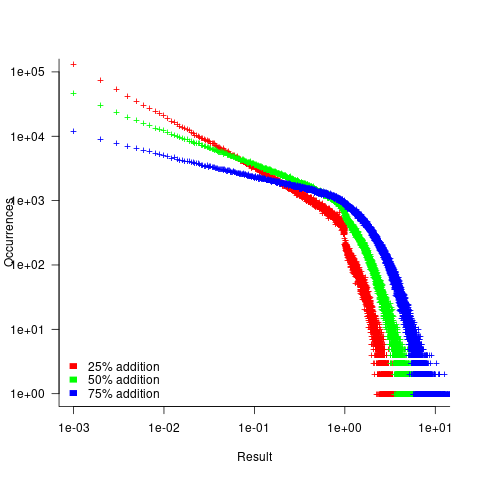
A rationale for the change in the slopes, for expressions containing different percentages of add/multiply, can be found in an earlier post looking at the distribution of many additions (the Irwin-Hall distribution, which tends to a Normal distribution), and many multiplications (integer power of a log).
- The result of many additions is to produce values that increase with the number of additions, and spread out (i.e., increasing variance).
- The result of many multiplications is to produce values that become smaller with the number of multiplications, and become less spread out.
Which recent application spends a huge amount of time adding/multiplying values in the range -1 to 1?
Large language models. Yes, under the hood they are all linear algebra; adding and multiplying large matrices.
LLM expressions are often evaluated using a half-precision floating-point type. In this 16-bit type, the exponent is biased towards supporting very small values, at the expense of larger values not being representable. While operations on a 10-bit significand will experience lots of quantization error, I suspect that the behavior seen above not noticeable change.
Distribution of uptimes for high-performance computing systems
Computers break down every now and again and this is a serious problem when an application needs runs on thousands of individual computers (nodes) plugged together; lots more hardware creates lots more opportunity for a failure that renders any subsequent calculations by working nodes possible wrong. The solution is checkpointing; saving the state of each node every now and again, and rolling back to that point when a failure occurs. Picking the optimal interval between checkpoints requires knowledge the distribution of node uptimes, what is it?
Short answer: Node uptimes have a negative binomial distribution, or at least five systems at the Los Alamos National Laboratory do.
The longer answer is below as another draft section from my book Empirical software engineering with R. As always comments and pointers to more data welcome. R code and data here.
Distribution of uptimes for high-performance computing systems
Today’s high-performance computing systems are created by connecting together lots of cpus. There is a hierarchy to the connection in that many cpus may populate a single board, several boards may be fitted into a rack unit, several rack units into a cabinet, lots of cabinets lined up in a row within a room and more than one room in a facility. A common operating unit is the node, effectively a computer on which an operating system is running (the actual hardware involved may be a single or multi processor cpu). A high-performance system is built from thousands of nodes and an application program may run on compute nodes from more than one facility.
With so many components, failures occur on a regular basis and long running applications need to recover from such failures if they are to stand a reasonable chance of ever completing.
Applications running on the systems installed at the Los Alamos National Laboratory create checkpoints at regular intervals, writing data needed to do a full restore to storage. When a failure occurs an application is restarted from its most recent checkpoint, one node failure causes all nodes to be rolled back to their most recent checkpoint (all nodes create their checkpoints at the same time).
A tradeoff has to be made between frequently creating checkpoints, which takes resources away from completing execution of the application but reduces the amount of lost calculation, and infrequent checkpoints, which diverts less resources but incurs greater losses when a fault occurs. Calculating the optimum checkpoint interval requires knowing the distribution of node uptimes and the following analysis attempts to find this distribution.
Data
The data comes from 23 different systems installed at the Los Alamos National Laboratory (LANL) between 1996 and 2005. The total failure count for most of the systems is of the order of a few hundred; there are five systems (systems 2, 16, 18, 19 and 20) that each have several thousand failures and these are the ones analysed here.
The data consists of failure records for every node in a system. A failure record includes information such as system id, node number, failure time, restored to service time, various hardware characteristics and possible root causes for the failure. Schroeder and Gibson <book Schroeder_06> performed the first analysis of the dataset and provide more background details.
Is the data believable?
Failure records are created by operations staff when they are notified by the automated monitoring system that a failure has been detected. Given that several people are involved in the process <book LANL_data_06> it seems unlikely that failures will go unreported.
Some of the failure reports have start times before the given node was returned into service from the previous failure; across the five systems this varied between 0.4% and 2.5%. It is possible that these overlapping failures are caused by an incorrectly attempt to fix the first failure, or perhaps they are data entry errors. This error rate is comparable with human error rates for low stress/non-critical work
The failure reports do not include any information about the application software running on the node when it failed; the majority of the programs executed are large-scale scientific simulations, such as simulations of nuclear stockpile stability. Thus it is not possible to accurately calculate the node MTBF for an executing application. LANL say <book LANL_data_06> that the applications “… perform long periods (often months) of CPU computation, interrupted every few hours by a few minutes of I/O for check-pointing.”
Predictions made in advance
The purpose of this analysis is to find the distribution that best fits the node uptime data, i.e., the time interval between failures of the same node.
Your author is not aware of any empirically based theory that predicts the uptime of high performance computing systems. The Poisson and exponential distributions are both frequently encountered in the analysis of hardware failures and it is always comforting to fit in with existing expectations.
Applicable techniques
A [Cullen and Frey test] matches a dataset’s skew and kurtosis against known distributions (in the case of the descdist function in the fitdistrplus package this is a handful of commonly encountered distributions); the fitdist function in the same package can be used to fit the data to a specified distribution.
Results
The table below lists some basic properties of each of the systems analysed. The large difference in mean/median uptimes between some systems is caused by very fat tails in the uptime distribution of some systems, see [LANL-node-uptime-binned].
| System | Nodes | Failures | Mean | Median |
|---|---|---|---|---|
|
2
|
49
|
6997
|
133
|
377
|
|
16
|
16
|
2595
|
89
|
229
|
|
18
|
823
|
3014
|
2336
|
4147
|
|
19
|
738
|
2344
|
2376
|
4069
|
|
20
|
323
|
2063
|
653
|
2544
|
If there are any significant changes in failure rate over time or across different nodes in a given system it could have a significant impact on the distribution of uptime intervals. So we first check to large differences in failure rates.
Do systems experience any significant changes in failure rate over time?
The plot below shows the total number of failures, binned using 30-day periods, for the five systems. Two patterns that stand out are system 20 which experienced many failures during the first few months and then settled down, and system 2’s sudden spike in failures around month 23 before settling down again. This analysis is intended to be broad brush and does not get involved with details of specific systems, but these changes in failure frequency suggest that the exact form of any fitted distribution may change over time in turn potentially leading to a change of checkpoint interval.
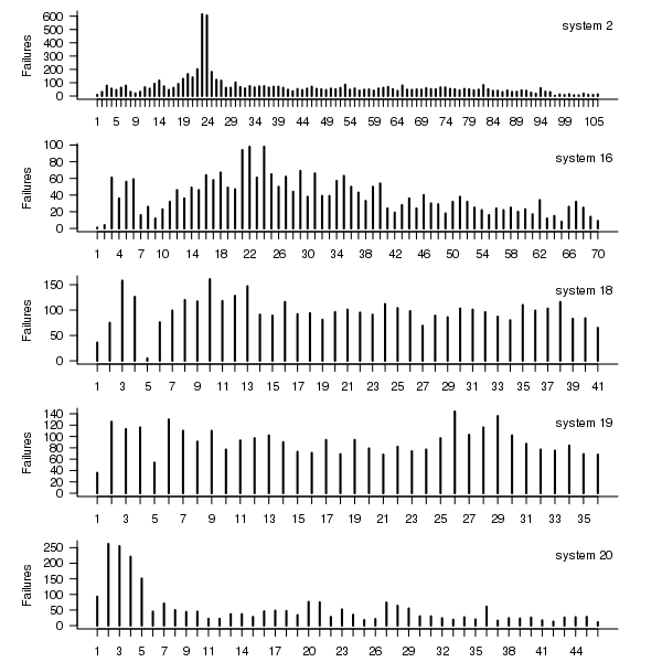
Figure 1. Total number of failures per 30-day interval for each LANL system.
Do some nodes failure more often than others?
The plot below shows the total number of failures for each node in the given system. Node 0 has many more failures than the other nodes (for node 0 of system 2 most of the failure data appears to be missing, so node 1 has the most failures). The distribution suggested by the analysis below is not changed if Node 0 is removed from the dataset.
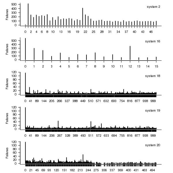
Figure 2. Total number of failures for each node in the given LANL system.
Fitting node uptimes
When plotted in units of 1 hour there is a lot of variability and so uptimes are binned into 10 hour units to help smooth the data. The number of uptimes in each 10-hour bin forms a discrete distribution and a [Cullen and Frey test] suggests that the negative binomial distribution might provide the best fit to the data; the Scroeder and Gibson analysis did not try the negative binomial distribution and of those they tried found the Weilbull distribution gave the best fit; the R functions were not able to fit this distribution to the data.
The plot below shows the 10-hour binned data fitted to a negative binomial distribution for systems 2 and 18. Visually the negative binomial distribution provides the better fit and the Akaiki Information Criterion values confirm this (see code for details and for the results on the other systems, which follow one of the two patterns seen in this plot).
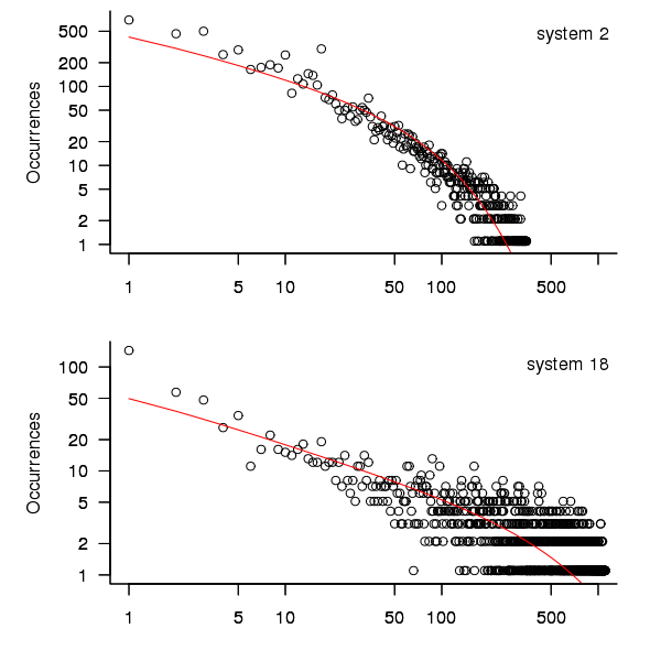
Figure 3. For systems 2 and 18, number of uptime intervals, binned into 10 hour interval, red line is fitted negative binomial distribution.
The negative binomial distribution is also the best fit for the uptime of the systems 16, 19 and 20.
The Poisson distribution often crops up in failure analysis. The quality of fit of a Poisson distribution to this dataset was an order of worse for all systems (as measured by AIC) than the negative binomial distribution.
Discussion
This analysis only compares how well commonly encountered distributions fit the data. The variability present in the datasets for all systems means that the quality of all fitted distributions will be poor and there is no theoretical justification for testing other, non-common, distributions. Given that the analysis is looking for the best fit from a chosen set of distributions no attempt was made to tune the fit (e.g., by forming a zero-truncated distribution).
Of the distributions fitted the negative binomial distribution has the lowest AIC and best fit visually.
As discussed in the section on [properties of distributions] the negative binomial distribution can be generated by a mixture of [Poisson distribution]s whose means have a [Gamma distribution]. Perhaps the many components in a node that can fail have a Poisson distribution and combined together the result is the negative binomial distribution seen in the uptime intervals.
The Weilbull distribution is often encountered with datasets involving some form of time between events but was not seen to be a good fit (for a continuous distribution) by a Cullen and Frey test and could not be fitted by the R functions used.
The characteristics of node uptime for two systems (i.e., 2 and 16) follows what might be thought of as a typical distribution of measurements, with some fattening in the tail, while two systems (i.e., 18 and 19) have very fat tails with indeed and system 20 sits between these two patterns. One system characteristic that matches this pattern is the number of nodes contained within it (with systems 2 and 16 having under 50, 18 and 19 having over 1,000 and 20 having around 500). The significantly difference in the size of the tails is reflected in the mean uptimes for the systems, given in the table above.
Summary of findings
The negative binomial distribution, of the commonly encountered distributions, gives the best fit to node uptime intervals for all systems.
There is over an order of magnitude variation in the mean uptime across some systems.
Developers do not remember what code they have written
The size distribution of software components used in building many programs appears to follow a power law. Some researchers have and continue to do little more than fit a straight line to their measurements, while those that have proposed a process driving the behavior (e.g., information content) continue to rely on plenty of arm waving.
I have a very simple, and surprising, explanation for component size distribution following power law-like behavior; when writing new code developers ignore the surrounding context. To be a little more mathematical, I believe code written by developers has the following two statistical properties:
- nesting invariance. That is, the statistical characteristics of code sequences does not depend on how deeply nested the sequence is within
if/for/while/switchstatements, - independent of what went immediately before. That is the choice of what statement a developer writes next does not depend on the statements that precede it (alternatively there is no short range correlation).
Measurements of C source show that these two properties hold for some constructs in some circumstances (the measurements were originally made to serve a different purpose) and I have yet to see instances that significantly deviate from these properties.
How does writing code following these two properties generate a power law? The answer comes from the paper Power Laws for Monkeys Typing Randomly: The Case of Unequal Probabilities which proves that Zipf’s law like behavior (e.g., the frequency of any word used by some author is inversely proportional to its rank) would occur if the author were a monkey randomly typing on a keyboard.
To a good approximation every non-comment/blank line in a function body contains a single statement and statements do not often span multiple lines. We can view a function definition as being a sequence of statement kinds (e.g., each kind could be if/for/while/switch/assignment statement or an end-of-function terminator). The number of lines of code in a function is closely approximated by the length of this sequence.
The two statistical properties listed above allow us to treat the selection of which statement kind to write next in a function as mathematically equivalent to a monkey randomly typing on a keyboard. I am not suggesting that developers actually select statements at random, rather that the set of higher level requirements being turned into code are sufficiently different from each other that developers can and do write code having the properties listed.
Switching our unit of measurement from lines of code to number of tokens does not change much. Every statement has a few common forms that occur most of the time (e.g., most function calls contain no parameters and most assignment statements assign a scalar variable to another scalar variable) and there is a strong correlation between lines of code and token count.
What about object-oriented code, do developers follow the same pattern of behavior when creating classes? I am not aware of any set of measurements that might help answer this question, but there have been some measurements of Java that have power law-like behavior for some OO features.
Recent Comments