Archive
Halstead/McCabe: a complicated formula for LOC
My experience is that people prefer to ignore the implications of Halstead’s metric and McCabe’s complexity metric being strongly correlated (non-linearly) with lines of code (LOC). The implications being that they have been deluding themselves and perhaps wasting time/money using Halstead/McCabe when they could just as well have used LOC.
If the purpose of collecting metrics is a requirement to tick a box, then it does not really matter which metrics are collected. The Halstead/McCabe metrics have a strong brand, so why not collect them.
Don’t make the mistake of thinking that Halstead/McCabe is more than a complicated way of calculating LOC. This can be shown by replacing Halstead/McCabe by the corresponding LOC value to find that it makes little difference to the value calculated.
Some metrics include the Halstead metrics and/or the McCabe metric as part of their calculation. The Maintainability Index is a metric calculated using Halstead’s volume, McCabe’s complexity and lines of code. Its equation is (see below for details):
-0.23*McCabe-16.2*ln(LOC)")
Replacing the Halstead/McCabe terms by one involving just LOC requires an appropriate mapping. Nearly all researchers assume a linear mapping, despite the overwhelming evidence that the mapping is non-linear.
Fitting regression models for HalsteadVolume vs LOC and McCabe vs LOC, using measurements of 730K methods from 47 Java projects (see below for data details), produces the coefficients for the equation needed to map each metric to LOC (previous analysis has found that a power law provides the best mapping; code+data). Substituting these equations in the Maintainability Index equation above, we get:
)-0.23*(0.45*LOC^{0.71})-16.2*ln(LOC)")
which simplifies to:
-0.1*LOC^{0.71}")
How does the value calculated using  compare with the corresponding
  value?
For 99.7% of methods, the relative error,  , for the 730K Java methods is less than 10%, and for 98.6% of methods the relative error is less than 5% (code+data).
Given the fuzzy nature of these metrics, 10% is essentially noise.
Looking at the relative contributions made by Halstead/McCabe/LOC to the value of the Maintainability Index, second equation above, the Halstead contribution is around a third the size of the LOC contribution and the McCabe contribution is at least an order of magnitude smaller.
Background on the Maintainability Index and the measured Java projects.
The Maintainability Index was introduced in the 1994 paper “Construction and Testing of Polynomials Predicting Software Maintainability” by Oman, and Hagemeister (270 citations; no online pdf), a 1992 paper by the same authors is often incorrectly cited (426 citations). The earlier 1992 paper identified 92 known maintainability attributes, along with 60 metrics for “… gauging software maintainability …” (extracted from 35 published papers).
This Maintainability Index equation was chosen from “Approximately 50 regression models were constructed and tested in our attempts to identify simple models that could be calculated from existing tools and still be generic enough to be applied to a wide range of software.” The data fitted came from eight suites of programs (average LOC 3,568 per suite), along “… with subjective engineering assessments of the quality and maintainability of each set of code.”
Yes, choosing from 50 regression models looks like overfitting, and by today’s standards 28.5K LOC is a tiny amount of source.
The data used is distributed with the paper Revisiting the Debate: Are Code Metrics Useful for Measuring Maintenance Effort? by Chowdhury, Holmes, Zaidman, and Kazman, which does a good job of outlining the many different definitions of maintenance and the inconsistent results from prediction models. However, the authors remain under the street light of project source code, i.e., they ignore the fact that many maintenance requests are driven by demand for new features.
The authors investigate the impact of normalizing Halstead/McCabe by LOC, but make the common mistake of assuming a linear relationship. They are surprised by the high correlation between post-‘normalised’ Halstead/McCabe and LOC. The correlation disappears when the appropriate non-linear normalization is used; see code+data.
A 2014 paper by Najm also maps the components of the Maintainability Index to LOC, but uses a linear mapping from the Halstead/McCabe terms to LOC, creating a equation whose behavior is noticeably different.
Frequency of non-linear relationships in software engineering data
Causality is an integral part of the developer mindset, and correlation is a common hammer that developers use for the analysis of data (usually the Pearson correlation coefficient).
The problem with using Pearson correlation to analyse software engineering data is that it calculates a measure of linear relationships, and software data is often non-linear. Using a more powerful technique would not only enable any non-linearity to be handled, it would also extract more information, e.g., regression analysis.
My impression is that power laws and exponential relationships abound in software engineering data, but exactly how common are they (and let’s not forget polynomial relationships, e.g., quadratics)?
I claim that my Evidence-based Software Engineering analyses all the publicly available software engineering data. How often do non-linear relationships occur in this data?
The data is invariably plotted, and often a regression model is fitted. A search of the data analysis code (written in R) located 996 calls to plot and 446 calls to glm (used to fit a regression model; shell script).
In calls to plot, the log argument can be used to specify that a log-scale be used for a given axis. When the data has an exponential distribution, I specified the appropriate axis to be log-scaled (18% of cases); for a power law, both axis were log-scaled (11% of cases).
In calls to glm, one or more of the formula variables may be log transformed within the formula. When the data has an exponential distribution, either the left-hand side of the formula is log transformed (20% of cases), or one of the variables on the right-hand side (9% of cases, giving 29% in total); for a power law both sides of the formula are log transformed (12% of cases).
Within a glm formula, variables can be raised to a power by enclosing the expression in the I function (the ^ operator has a special meaning within a formula, but its usual meaning inside I). The most common operation appearing inside I is ^2, i.e., squaring a value. In the following table, only formula that did not log transform any variable were searched for calls to I.
The analysis code contained 54 calls to the nls function, whose purpose is to fit non-linear regression models.
    plot   log="x"  log="y"       log="xy"
    996      4%       14%            11%

    glm    log(x)   log(y)    log(y) ~ log(x)   I()
446 9% 20% 12% 12% |
Based on these figures (shell script), at least 50% of software engineering data contains non-linear relationships; the values in this table are a lower bound, because variables may have been transformed outside the call to plot or glm.
The at least 50% estimate is based on all software engineering, some corners will have higher/lower likelihood of encountering non-linear data; for instance, estimation data often contains power law relationships.
Correlation between risk attitude and willingness to refer back
What is the connection between a software developer’s risk attitude and the faults they insert in code they write or fail to detect in code they review? This is a very complicated question and in an experiment performed at the 2011 ACCU conference I investigated one particular instance; the connection between risk attitude and recall of previously seen information.
The experiment consisted of a series of problems having the same format (the identifiers used varied between problems). Each problem involved remembering information on four assignment statements of the form:
p = 6 ; b = 4 ; r = 9 ; k = 8 ; |
performing some other unrelated task for a short time (hopefully long enough for them to forget some of the information they had previously seen) and then having to recognize the variables they had previously seen within a list containing five identifiers and recall the numeric value assigned to each variable.
When reading code developers have the option of referring back to previously read code and this option was provided to subject. Next to each identifier listed in the recall part of the problem was space to write the numeric value previously seen and a “would refer back” box. Subjects were told to tick the “would refer back” box if, in real life” they would refer back to the previously seen assignment statements rather than rely on their memory.
As originally conceived this experimental format is investigating the impact of human short term memory on recall of previously seen code. Every time I ran this kind of experiment there was a small number of subjects who gave a much higher percentage of “would refer back” answers than the other subjects. One explanation was that these subjects had a smaller short term memory capacity than other subjects (STM capacity does vary between people), another explanation is that these subjects are much more risk averse than the other subjects.
The 2011 ACCU experiment was designed to test the hypothesis that there was a correlation between a subject’s risk attitude and the percentage of “would refer back” answers they gave. The Domain-Specific Risk-Taking (DOSPERT) questionnaire was used to measure subject’s risk attitude. This questionnaire and the experimental findings behind it have been published and are freely available for others to use. DOSPERT measures risk attitude in six domains: social, recreation, gambling, investing health and ethical.
The following scatter plot shows each (of 30) subject’s risk attitude in the six domains (x-axis) plotted against percentage of “would refer back” answers (y-axis).
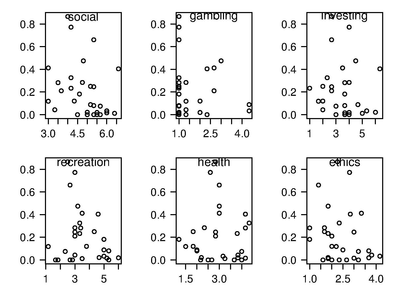
A Spearman rank correlation test confirms what is visibly apparent, there is no correlation between the two quantities. Scatter plots using percentage of correct answers and total number of questions answers show a similar lack of correlation.
The results suggest that risk attitude (at least as measured by DOSPERT) is not a measurable factor in subject recall performance. Perhaps the subjects that originally caught my attention (there were three in 2011) really do have a smaller STM capacity compared to other subjects. The organization of the experiment (one hour during a one lunchtime of the conference) does not allow for a more extensive testing of subject cognitive characteristics.
Halstead’s metrics and flat-Earthers are still with us
I recently discovered a fascinating series of technical reports from the 1970s in the Purdue University e-Pubs archive that shine a surprising light on what are now known as the Halstead metrics.
The first surprises came from Halstead’s A Software Physics Analysis of Akiyama’s Debugging Data; surprising in the size of the data set used (nine measurements of four attributes), the amount of hand waving used to pluck numbers out of thin air, the substantial difference between the counting methods used then and now and the very high correlation found between various measured and calculated attributes.
I disagreed with the numbers Halstead plucked and wrote some R to check Halstead’s results and try out my own numbers. While my numbers significantly changed the effort estimation values, the high correlations between the number of faults and various source attributes remained high. Even changing from the Pearson correlation coefficient (calculating confidence bounds for this coefficient requires that the data be normally distributed, which it is not {program size is now thought to follow a power law/exponential like distribution}) to the Spearman rank correlation coefficient did not have much impact. Halstead seems to have struck luck with this data set.
What did Halstead’s colleagues at Purdue think of these metrics? The report Software Science Revisited: A Critical Analysis of the Theory and Its Empirical Support written four years after Halstead’s flurry of papers contains a lot of background material and points out the lack of any theoretical foundation for some of the equations, that the analysis of the data was weak and that a more thorough analysis suggests theory and data don’t agree. Damming stuff.
If it is known that Halstead’s metrics do not hold up why do writers of books (including Shen, Conte and Dunsmore, the authors of the above report) continue to discuss Halstead’s work? Are they treating this work like Astronomy authors treat Ptolemy’s theory (the Sun and planets revolved around the Earth), i.e., incorrect but part of history and worth a mention?
An observation in the Shen et al report, that Halstead originally proposed the metrics as a way of measuring the complexity of algorithms not programs, explains the background to the report Impurities Found in Algorithm Implementations. Halstead uses the term “impurities” and talks about the need for “purification” in his early work. In this report Halstead points out that the value of metrics for “algorithms written by students” are very different from those for the equivalent programs published in journals and goes on to list eight classes of impurity that need to be purified (i.e., removing or rewriting clumsy, inefficient or duplicate code) in order to obtain results that agree with the theory. Now we know what needs to be done to existing programs to get them to agree with the predictions made by the Halstead metrics!
Did Halstead strike lucky with the data used in his first published analysis of ‘industrial code’, obtaining a very high correlation that caused him to shift focus away from measuring algorithms to measuring programs? Unfortunately, he died soon after publishing the work for which he is now known, so he did not get to comment on how his ideas were used over the subsequent years.
Why are people still attracted to the Halstead metrics, given their poor theoretical foundations and a predictive power that is comparable with using lines of code? Is it because the idea of code volume and length are easy to understand and so are attractive (dimensionally, both of these metrics are the same, a fact that cannot hold for any self-consistent concept of volume and length)? Is it because we don’t have alternative metrics that outperform the poorly performing ones proposed by Halstead, after all Copernicus only won out because his theory gave answers that were more accurate than Ptolomy’s.
Perhaps like the flat Earthers proponents of the Halstead metrics will always be with us.
Developers do not remember what code they have written
The size distribution of software components used in building many programs appears to follow a power law. Some researchers have and continue to do little more than fit a straight line to their measurements, while those that have proposed a process driving the behavior (e.g., information content) continue to rely on plenty of arm waving.
I have a very simple, and surprising, explanation for component size distribution following power law-like behavior; when writing new code developers ignore the surrounding context. To be a little more mathematical, I believe code written by developers has the following two statistical properties:
- nesting invariance. That is, the statistical characteristics of code sequences does not depend on how deeply nested the sequence is within
if/for/while/switchstatements, - independent of what went immediately before. That is the choice of what statement a developer writes next does not depend on the statements that precede it (alternatively there is no short range correlation).
Measurements of C source show that these two properties hold for some constructs in some circumstances (the measurements were originally made to serve a different purpose) and I have yet to see instances that significantly deviate from these properties.
How does writing code following these two properties generate a power law? The answer comes from the paper Power Laws for Monkeys Typing Randomly: The Case of Unequal Probabilities which proves that Zipf’s law like behavior (e.g., the frequency of any word used by some author is inversely proportional to its rank) would occur if the author were a monkey randomly typing on a keyboard.
To a good approximation every non-comment/blank line in a function body contains a single statement and statements do not often span multiple lines. We can view a function definition as being a sequence of statement kinds (e.g., each kind could be if/for/while/switch/assignment statement or an end-of-function terminator). The number of lines of code in a function is closely approximated by the length of this sequence.
The two statistical properties listed above allow us to treat the selection of which statement kind to write next in a function as mathematically equivalent to a monkey randomly typing on a keyboard. I am not suggesting that developers actually select statements at random, rather that the set of higher level requirements being turned into code are sufficiently different from each other that developers can and do write code having the properties listed.
Switching our unit of measurement from lines of code to number of tokens does not change much. Every statement has a few common forms that occur most of the time (e.g., most function calls contain no parameters and most assignment statements assign a scalar variable to another scalar variable) and there is a strong correlation between lines of code and token count.
What about object-oriented code, do developers follow the same pattern of behavior when creating classes? I am not aware of any set of measurements that might help answer this question, but there have been some measurements of Java that have power law-like behavior for some OO features.
Recent Comments