Archive
Extracting numbers from a stacked density plot
A month or so ago, I found a graph showing a percentage of PCs having a given range of memory installed, between March 2000 and April 2020, on a TechTalk page of PC Matic; it had the form of a stacked density plot. This kind of installed memory data is rare, how could I get the underlying values (a previous post covers extracting data from a heatmap)?
The plot below is the image on PC Matic’s site:
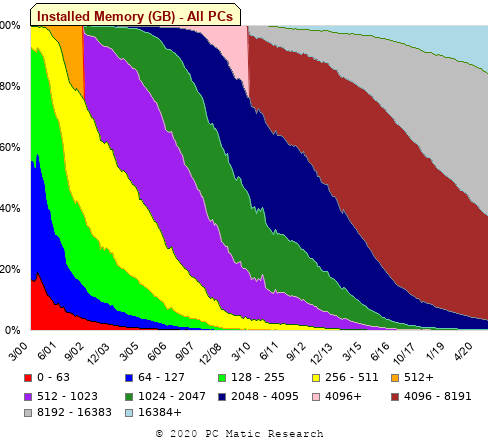
The change of colors creates a distinct boundary between different memory capacity ranges, and it ought to be possible to find the y-axis location of each color change, for a given x-axis location (with location measured in pixels).
The image was a png file, I loaded R’s png package, and a call to readPNG created the required 2-D array of pixel information.
library("png")
img=readPNG("../rc_mem_memrange_all.png") |
Next, the horizontal and vertical pixel boundaries of the colored data needed to be found. The rectangle of data is surrounded by white pixels. The number of white pixels (actually all ones corresponding to the RGB values) along each horizontal and vertical line dramatically drops at the data image boundary. The following code counts the number of col points in each horizontal line (used to find the y-axis bounds):
horizontal_line=function(a_img, col)
{
lines_col=sapply(1:n_lines, function(X) sum((a_img[X, , 1]==col[1]) &
                                            (a_img[X, , 2]==col[2]) &
                                            (a_img[X, , 3]==col[3]))
                )

return(lines_col)
}

white=c(1, 1, 1)
n_cols=dim(img)[2]

# Find where fraction of white points on a line changes dramatically
white_horiz=horizontal_line(img, white)

# handle when upper boundary is missing
ylim=c(0, which(abs(diff(white_horiz/n_cols)) > 0.5))
ylim=ylim[2:3] |
Next, for each vertical column of pixels, at each x-axis pixel location, the sought after y value occurs at the change of color boundary in the corresponding vertical column. This boundary includes a 1-pixel wide separation color, which creates a run of 2 or 3 consecutive pixel color changes.
The color change is easily found using the duplicated function.
# Return y position of vertical color changes at x_pos
y_col_change=function(x_pos)
{
# Good enough technique to generate a unique value per RGB color
col_change=which(!duplicated(img[y_range, x_pos, 1]+
                          10*img[y_range, x_pos, 2]+
                         100*img[y_range, x_pos, 3]))

# Handle a 1-pixel separation line between colors.
# Diff is used to find these consecutive sequences.
y_change=c(1, col_change[which(diff(col_change) > 1)+1])

# Always return a vector containing max_vals elements.
return(c(y_change, rep(NA, max_vals-length(y_change))))
} |
Next, we need to group together the sequence of points that delimit a particular boundary. The points along the same boundary are all associated with the same two colors, i.e., the ones below/above the boundary (plus a possible boundary color).
The plot below shows all the detected boundary points, in black, overwritten by colors denoting the points associated with the same below/above colors (code):

The visible black pluses show that the algorithm is not perfect. The few points here and there can be ignored, but the two blocks at the top of the original image have thrown a spanner in the works for some range of points (this could be fixed manually, or perhaps it is possible to tweak the color extraction formula to work around them).
How well does this approach work with other stacked density plots? No idea, but I am on the lookout for other interesting examples.
Code generation via machine learning
Commercial compiler implementors have to produce compilers that are capable of being used on a typical developer computer. A whole bunch of optimization techniques were known for years but could not be used because few computers had the available memory capacity (in the days when 2M was a lot of memory your author once attended a talk that presented some impressive results and was frustrated to learn that the typical memory footprint was 160M, who would ever imagine developers having so much memory to work within?) These days the available of gigabytes of storage has means that likely computer storage capacity is rarely a reason not to use some optimization technique, although the whole program optimization people are still out in the cold.
What is new these days is the general availability of multiple processors. The obvious use of multiple processors is to have make distribute the compilation load. The more interesting use is having the compiler apply different sets of optimizations techniques on different processors, picking the one that produces the highest quality code.
Optimizing code generation algorithms don’t appear to leave anything to chance and individually they generally don’t. However, selecting an order in which to apply individual optimization algorithms is something of a black art. In some cases code transformations made by one algorithm can interfere with the performance of another algorithm. In some cases the possibility of the interference is known and applies in one direction, choosing the appropriate relative ordering of the two algorithms solves the problem. In other cases the way in which two algorithms interfere with each other depends on the code being translated, now the ordering of the two algorithms becomes problematic. The obvious solution is to try both orderings and pick the one that produces the best result.
Several research groups have investigated the use of machine learning in compiler optimization. cTuning.org is a new project that aims to bring together groups interested in self-tuning adaptive computing systems based on statistical and machine learning techniques.
Commercial pressure is always forcing compiler implementors to produce faster code and use of machine learning techniques can produce some impressive results. Now that multi-processor systems are common it will not be long before compilers writers start to make use of the extra resources now available to them.
The safety critical people have problems trying to show the correctness of compiler output that has been generated by ‘fixed’ algorithms. It is not hard to envisage that in 10 years time all large production quality compilers will be using machine learning.
Recent Comments