Archive
Accuracy of Function Point estimates
The number of Function points, FP, contained in the implementation of a software system are counted by following a specified counting process. The number of FP counted for a project is mapped to a cost estimate by multiplying the number of FP by the predetermined cost value of one FP; the predetermined value is based on cost data from similar previous projects within the company. The FP process is so popular as a unit of cost estimation that there are six different ISO standards specifying six different Function point measurement processes.
TL;DR: Estimated cost is not as accurate as traditional time based estimating, although the estimation process may produce consistent FP counts.
The FP certification schemes run by various organizations require applicants to pass exams that check they are consistently following the specified processes to produce consistent FP counts, i.e., that certified practitioners give very similar answers for the same implementation problem. Experiments where subjects used different counting processes to count FP for the same task, have found what looks like a linear relationship between various pairs of FP counting processes.
Having certified FP employees/consultants produce similar counts is all well and good, but what management actually wants is a close correspondence between estimated and actual costs. What does the available data show with regard to FP cost estimation accuracy?
I know of two FP/Cost datasets, one containing 149 points from one company (actual costs have been normalised), and the other 492 points from three companies (actual costs in Euros; FP used is IFPUG); this dataset also includes additional context information and is used in this post’s analysis.
What is the relationship between an estimate based on FP and actual cost? The plot below show FP against actual cost, the red line is the fitted regression equation  , the grey line shows
  (code+data):
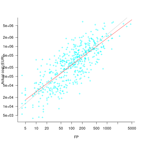
The power law exponent, 0.8, is slightly smaller than the 0.85 value found when fitting time estimates to actual times.
The dataset includes information specifying: anonymous organization ID, development method (78.5% plan driven and 21.5% Scrum), business domain (e.g., Call center, Mortgages, Front office), and various 0/1 flags each denoting a particular characteristic.
Including this information in a regression model finds that some of them have an impact on the FP to actual cost mapping. This is not surprising, since the FP/cost mapping is intended to be based on similar previous projects. The fitted model has the form:

where:  ,
,  ,
,  , and
, and  are constants for the corresponding items from the fitted regression model.
The fitted value for the scrum the development method is  , and
, and  for plan based (i.e., waterfall), i.e., Agile FP are cheaper than Waterfall FP. The idea of using both FP and scrum had not crossed my mind. Estimating via FP requires a detailed breakdown of the work to be done, while scrum is a process that discovers the work to be done. Perhaps a scrum like methodology was used to implement the detailed breakdown used to count FPs. The apparent lower cost of scrum FPs could just be a result of discovering that some planned functionality was not required.
How accurate were the FP estimates?
It is not possible to answer this question between we don’t know the cost assigned to one FP; in the above plot, the grey lines shows  .
.
We can calculate an estimate accuracy relative to the fitted model (the red line above). The mapping from FP to cost can vary between organizations, and the following analysis is based on the data for each distinct organization. The plot below shows the points, and associated fitted regression line, for the three organizations (code+data):
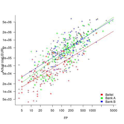
Each organization’s fitted regression model can be used to calculate confidence intervals. Approximately 68% of FP estimates could be off by over a factor two (between 2.3 and 2.5) from the mean actual cost, while for the 95% interval FP estimates could be off by over a factor five (it varied between 5.0 and 5.8); code+data. The corresponding factors for traditional developer time estimation are two and four.
The exponent varies between 0.72 and 0.84, with Beltel and Bank B having very similar values (the exponent for time estimates is often close to 0.85). The FP/Cost mapping is likely to be similar for the two banks, but lower for the telecoms company.
Does slicing the data by organization and business domain reduce the width of the confidence intervals, i.e., smaller multiplication factor? In some cases the width is reduced, but in other cases the width is increased; the 68% factor is between 1.9 and 3.1, the 95% factor is between 3.2 and 9.4.
Evaluating Story point estimation error
If a task implementation estimate is expressed in time, various formula are available for evaluating how well the estimated time corresponds to the actual time.
When an estimate is expressed in story points, how might the estimate be evaluated when actual time is measured in hours?
The common practice of selecting story point values from a small set of integers (I have seen fractional values used) introduces quantization error into most estimates (around 30% of time estimates equal actual time), assuming that actual times are not constrained to a similar number of possible time values.
If we assume a linear mapping from estimated story points to actual time and an ideal estimator (let’s assume that 1 story point is equivalent to 1 hour), then a lower bound on the error can be calculated.
Our ideal estimator is able to exactly predict the actual time. However, the use of story points means that this exact prediction has to be rounded to one of a small set of integer values. Let’s assume that our ideal estimator rounds to the story point value that is closest to the exact prediction, e.g., all story points predicted to take up to 1.5 are estimated at 1 story point.
What is the mean error of the estimates made by this ideal, rounded, estimator?
The available evidence shows that the distribution of tasks having a given actual implementation time roughly has the form of a geometric (the discrete form of exponential) or negative binomial distribution. The plot below shows a geometric and negative binomial distribution, with distinct colors over the range where values are rounded to the same closest integer (dots are at 1-minute intervals, code):
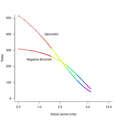
Having picked a distribution for actual times, we can calculate the number of tasks estimated to require, for instance, 1 story point, but actually taking 1 hour, 1 hr 1 min, 1 hr 2 min, …, 1 hr 30 min. The mean error can be calculated over each pair of estimate/actual, for one to five story points (in this example). The table below lists the mean error for two actual distributions, calculated using four common metrics: squared error (SE), absolute error (AE), absolute percentage error (APE), and relative error (RE); code:
Distribution SE AE APE RE Geometric 0.087 0.26 0.17 0.20 Negative Binomial 0.086 0.25 0.14 0.16 |
A few minutes difference in a 1 SP estimate is a larger error than the same number of minutes in a two or more SP estimate, combined with most tasks take a small amount of time, means that error estimation is dominated by inaccuracies in estimating small tasks.
In practice, the range of actual times, for a given estimate, is better approximated by a percentage of the estimated time (50% is used below), and the number of tasks having a given actual value for a given estimate, approximated by a triangular distribution (a cubic equation was used for the following calculation). The plot below shows the distribution of estimation points around a given number of story points (at 1-minute intervals), and the geometric and negative binomial distribution (compare against plot above to work out which is which; code):
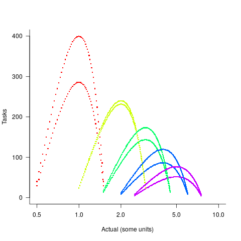
The following table lists of mean errors:
Distribution SE AE APE RE Geometric 0.52 0.55 0.13 0.13 Negative Binomial 0.62 0.61 0.13 0.14 |
When the error in the actual is a percentage of the estimate, larger estimates have a much larger impact on absolute accuracy; see the much larger SE and AE values. The impact on the relative accuracy metrics appears to be small.
Is evaluating estimation error useful, when estimates are given in story points?
While it’s possible to argue for and against, the answer is that usefulness is in the eye of the beholder. If development teams find the information useful, then it is useful; otherwise not.
Over/under estimation factor for ‘most estimates’
When asked to estimate the time taken to perform a software development related task, people regularly over or under estimate. What range of over/under estimation falls within the bounds of the term ‘most estimates’, i.e., the upper/lower bounds of the ratio  (an overestimate occurs when
  , an underestimate when
  )?
)?
On Twitter, I have been citing a factor of two for over/under time estimates. This factor of two involves some assumptions and a personal interpretation.
The following analysis is based on the two major software task effort estimation datasets: SiP and CESAW. The tasks in both datasets are for internal projects (i.e., no tendering against competitors), and require at most a few hours work.
The following analysis is based on the SiP data.
Of the 8,252 unique tasks in the SiP data, 30% are underestimates, 37% exact, and 33% overestimates.
How do we go about calculating bounds for the over/under factor of most estimates (a previous post discussed calculating an accuracy metric over all estimates)?
A simplistic approach is to average over each of the overestimated and underestimated tasks. The plot below shows hours estimated against the ratio actual/estimated, for each task (code+data):
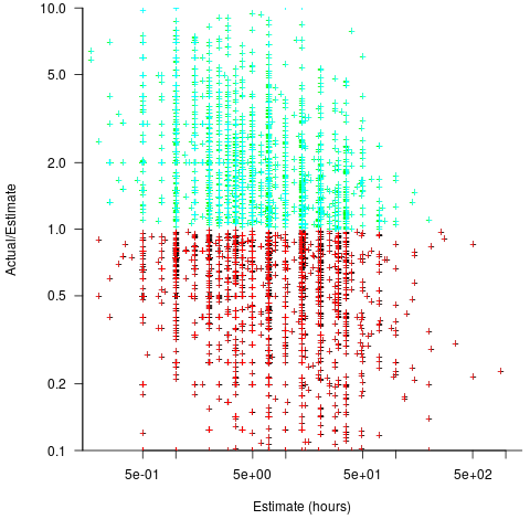
Averaging the over/under estimated tasks separately (using the geometric mean) gives 0.47 and 1.9 respectively, i.e., tasks are over/under estimated by a factor of two.
This approach fails to take into account the number of estimates that are over/under/equal, i.e., it ignores likelihood information.
A regression model takes into account the distribution of values, and we could adopt the fitted model’s prediction interval as the over/under confidence intervals. The prediction interval is the interval within which other observations are expected to fall, with some probability (R’s predict function uses one standard deviation).
The plot below shows a fitted regression model and prediction intervals at one standard deviation (68.3%) and two standard deviations (95%); the faint grey line shows Estimate == Actual (code+data):
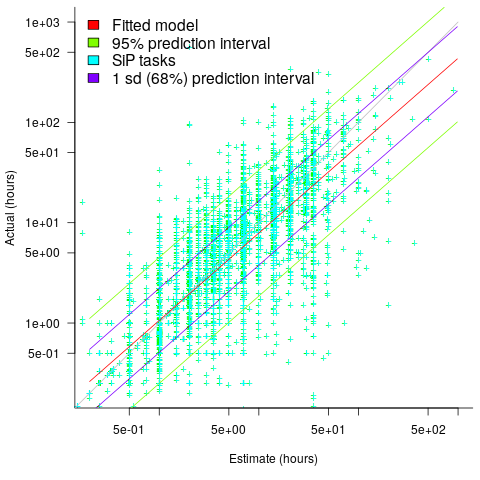
The fitted model tilts down from the upward direction of the Estimate == Actual line, consequently the over/under estimation factor depends on the size of the estimate. The table below lists the over/under estimation factor for low/high estimates at one & two standard deviations (68.3 and 95% probability).
People like simple answers (i.e., single values) and the mean value is a commonly used technique of summarising many values. The task estimate values are unevenly distributed and weighting the mean by the distribution of estimated values is more representative than, say, an evenly distributed set of estimates. The 5th and 6th columns in the table below list the weighted means at one/two standard deviations (the CESAW columns are the values for all projects in the CESAW data).
          1 sd           2 sd        Weighted mean       CESAW
       Low    High   Low    High     1 sd    2 sd     1 sd   2 sd
Over   0.56   0.24   0.27   0.11     0.46    0.25     0.29   0.1
Under 2.4 1.0 4.9 2.0 2.00 4.1 2.4 6.5 |
The weighted means for over/under estimates are close to a factor of two of the actual (divide/multiply) within one standard deviation (68.3%), and a factor of four within two standard deviations (95%).
Why choose to give the one standard deviation factor, rather than the two? People talk of “most estimates”, but what percentage range does ‘most’ map to? I have tended to think of ‘most’ as more than two-thirds, e.g., at least one standard deviation (a recent study suggests that ‘most’ usage peaks at 80-85%), and I think of two standard deviations as ‘nearly all’ (i.e., 95%; there are probably people who call this ‘most’).
Perhaps a between two and four is a more appropriate answer (particularly since the bounds are wider for the CESAW data). Suggestions welcome.
Another nail for the coffin of past effort estimation research
Programs are built from lines of code written by programmers. Lines of code played a starring role in many early effort estimation techniques (section 5.3.1 of my book). Why would anybody think that it was even possible to accurately estimate the number of lines of code needed to implement a library/program, let alone use it for estimating effort?
Until recently, say up to the early 1990s, there were lots of different computer systems, some with multiple (incompatible’ish) operating systems, almost non-existent selection of non-vendor supplied libraries/packages, and programs providing more-or-less the same functionality were written more-or-less from scratch by different people/teams. People knew people who had done it before, or even done it before themselves, so information on lines of code was available.
The numeric values for the parameters appearing in models were obtained by fitting data on recorded effort and lines needed to implement various programs (63 sets of values, one for each of the 63 programs in the case of COCOMO).
How accurate is estimated lines of code likely to be (this estimate will be plugged into a model fitted using actual lines of code)?
I’m not asking about the accuracy of effort estimates calculated using techniques based on lines of code; studies repeatedly show very poor accuracy.
There is data showing that different people implement the same functionality with programs containing a wide range of number of lines of code, e.g., the 3n+1 problem.
I recently discovered, tucked away in a dataset I had previously analyzed, developer estimates of the number of lines of code they expected to add/modify/delete to implement some functionality, along with the actuals.
The following plot shows estimated added+modified lines of code against actual, for 2,692 tasks. The fitted regression line, in red, is:  (the standard error on the exponent is
  ), the green line shows
  (code+data):
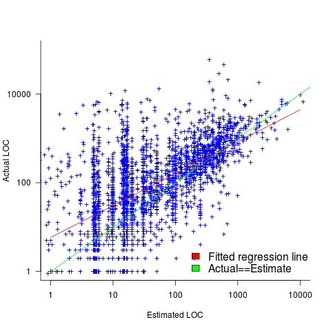
The fitted red line, for lines of code, shows the pattern commonly seen with effort estimation, i.e., underestimating small values and over estimating large values; but there is a much wider spread of actuals, and the cross-over point is much further up (if estimates below 50-lines are excluded, the exponent increases to 0.92, and the intercept decreases to 2, and the line shifts a bit.). The vertical river of actuals either side of the 10-LOC estimate looks very odd (estimating such small values happen when people estimate everything).
My article pointing out that software effort estimation is mostly fake research has been widely read (it appears in the first three results returned by a Google search on software fake research). The early researchers did some real research to build these models, but later researchers have been blindly following the early ‘prophets’ (i.e., later research is fake).
Lines of code probably does have an impact on effort, but estimating lines of code is a fool’s errand, and plugging estimates into models built from actuals is just crazy.
Initial impressions of RangeLab
I was rummaging around in the source of R looking for trouble, as one does, when I came across what I believed to be a less than optimally accurate floating-point algorithm (function R_pos_di in src/main/arithemtic.c). Analyzing the accuracy of floating-point code is notoriously difficult and those having the required skills tend to concentrate their efforts on what are considered to be important questions. I recently discovered RangeLab, a tool that seemed to be offering painless floating-point code accuracy analysis; here was an opportunity to try it out.
Installation went as smoothly as newly released personal tools usually do (i.e., some minor manual editing of Makefiles and a couple of tweaks to the source to comment out function calls causing link errors {mpfr_random and mpfr_random2}).
RangeLab works by analyzing the flow of values through a program to produce the set of output values and the error bounds on those values. Input values can be specified as a range, e.g., f = [1.0, 10.0] says f can contain any value between 1.0 and 10.0.
My first RangeLab program mimicked the behavior of the existing code in R_pos_di:
n=-10; f=[1.0, 10.0]; res = 1.0; if n < 0, n = -n; f = 1 / f; end while n ~= 0, if (n / 2)*2 ~= n, res = res * f; end n = n / 2; if n ~= 0, f = f*f; end end |
and told me that the possible range of values of res was:
res ans = float64: [1.000000000000001E-10,1.000000000000000E0] error: [-2.109423746787798E-15,2.109423746787799E-15] |
Changing the code to perform the divide last, rather than first, when the exponent is negative:
n=-10; f=[1.0, 10.0]; res = 1.0; is_neg = 0; if n < 0, n = -n; is_neg = 1 end while n ~= 0, if (n / 2)*2 ~= n, res = res * f end n = n / 2; if n ~= 0, f = f*f end if is_neg == 1, res = 1 / res end end |
and the error in res is now:
res ans = float64: [1.000000000000000E-10,1.000000000000000E0] error: [-1.110223024625156E-16,1.110223024625157E-16] |
Yea! My hunch was correct, moving the divide from first to last reduces the error in the result. I have reported this code as a bug in R and wait to see what the R team think.
Was the analysis really that painless? The Rangelab language is somewhat quirky for no obvious reason (e.g., why use ~= when everybody uses != these days and if conditionals must be followed by a character why not use the colon like Python does?) It would be real useful to be able to cut and paste C/C++/etc and only have to make minor changes.
I get the impression that all the effort went into getting the analysis correct and user interface stuff was a very distant second. This is the right approach to take on a research project. For some software to make the leap from interesting research idea to useful tool it is important to pay some attention to the user interface.
The current release does not deserve to be called 1.0 and unless you have an urgent need I would suggest waiting until the usability has been improved (e.g., error messages give some hint about what is wrong and a rough indication of which line the problem occurs on).
RangeLab has shown that there is simpler method of performing useful floating-point error analysis. With some usability improvements RangeLab would be an essential tool for any developer writing code involving floating-point types.
Update: The R team, in the form of Martin Maechler, resolved my report in just over 14 hours! The function R_pos_di is not called, the pow function from the C library (which takes two double arguments rather than a double and an int) has been found to be more accurate. Martin says this usage is not less accurate even for n=3, which I find surprising; I agree it should be more accurate for large values of n.
pow is one of the more complicated maths functions, involving finding a log, a multiply and then returning the exponent of this result. There are lots of boundary values that need to be checked and the code goes on for a while. I will wait for the usability of RangeLab to improve before attempting to compare its accuracy against the simpler algorithm for integer powers. Looking at the SunOracle library sources, if both arguments have integral values the ‘integer power’ algorithm is used (with the divide performed last).
Automatically improving code
Compared to 20 or 30 years ago we know a lot more about the properties of algorithms and better ways of doing things often exist (e.g., more accurate, faster, more reliable, etc). The problem with this knowledge is that it takes the form of lots and lots of small specific details, not the kind of thing that developers are likely to be interested in, or good at, remembering. Rather than involve developers in the decision-making process, perhaps the compiler could figure out when to substitute something better for what had actually been written.
While developers are likely to be very happy to see what they have written behaving as accurately and reliably as they had expected (ignorance is bliss), there is always the possibility that the ‘less better’ behavior of what they had actually written had really been intended. The following examples illustrate two relatively low level ‘improvement’ transformations:
- this case is probably a long-standing fault in many binary search and merge sort functions; the relevant block of developer written code goes something like the following:
while (low <= high)
   {
   int mid = (low + high) / 2;
   int midVal = data[mid];

   if (midVal < key)
      low = mid + 1
   else if (midVal > key)
      high = mid - 1;
   else
      return mid;
   }
The fault is in the expression
(low + high) / 2which overflows to a negative value, and returns a negative value, if the number of items being sorted is large enough. Alternatives that don’t overflow, and that a compiler might transform the code to, include:low + ((high - low) / 2)and(low + high) >>> 1. - the second involves summing a sequence of floating-point numbers. The typical implementation is a simple loop such as the following:
sum=0.0;
for i=1 to array_len
   sum += array_of_double[i];
which for large arrays can result in
sumlosing a great deal of accuracy. The Kahan summation algorithm tries to take account of accuracy lost in one iteration of the loop by compensating on the next iteration. If floating-point numbers were represented to infinite precision the following loop could be simplified to the one above:sum=0.0; c=0.0; for i = 1 to array_len { y = array_of_double[i] - c; // try to adjust for previous lost accuracy t = sum + y; c = (t - sum) - y; // try and gets some information on lost accuracy sum = t; }
In this case the additional accuracy is bought at the price of a decrease in performance.
Compiler maintainers are just like other workers in that they want to carry on working at what they are doing. This means they need to keep finding ways of improving their product, or at least improving it from the point of view of those willing to pay for their services.
Many low level transformations such as the above two examples would be not be that hard to implement, and some developers would regard them as useful. In some cases the behavior of the code as written would be required, and its transformed behavior would be surprising to the author, while in other cases the transformed behavior is what the developer would prefer if they were aware of it. Doesn’t it make sense to perform the transformations in those cases where the as-written behavior is least likely to be wanted?
Compilers already do things that are surprising to developers (often because the developer does not fully understand the language, many of which continue to grow in complexity). Creating the potential for more surprises is not that big a deal in the overall scheme of things.
Quality comparison of floating-point maths libraries
What is the best way to compare the quality of floating-point math libraries (e.g., sin, cos and log)? The traditional approach for evaluating the quality of an algorithm implementing a mathematical function is based on mathematics; methods have been developed to calculate the maximum error between the calculated and the actual value. The answer produced by this approach does not say anything about how frequently this maximum error will occur, only that it occurs at least once.
The log (natural logarithm) is probably the most frequently used mathematical function and I decided to compare a few implementations; R statistical package version 2.11.1 and glibc (libm version 2.11.2) both running under Suse 11.3 on an AMD Athlon 64 X2, and Cygwin version 1.7.1 under Windows XP SP 2 on another AMD Athlon 64 X2.
The algorithm often used to implement mathematical functions involves evaluating a polynomial expression (e.g., Chebyshev polynomials) within a small range of values (various methods are used to map the argument into this range and then scale the calculated result). I decided to initially treat the implementations under test as black boxes and did not know the ranges they used; a range of 0.1 to 1.0 seemed like a good idea and I generated all single precision floating-point values between these two bounds (all 28,521,267 of them, with each adjacent pair still having  double precision values between them).
#include <math.h> #include <stdio.h> int main(int argc, char *argv[]) { float val = 0.1, max_val = 1.0; while (val < max_val) { printf("%12.10f\n", val); val=nextafterf(val, 1.1); } } |
This list of 28 million values was fed as input to three programs:
- bc, which was used to generate the list of assumed to be correct logarithm of these 28 million values. R supports 64-bit IEEE compliant floating-point values, as do the C compilers/libraries used, and the number of decimal digits supported in this representation is 15. To provide greater accuracy to compare against the values generated by bc contained 17 digits, an extra two decimal digits over the IEEE values.
scale=17
while ((val=read() > 0))
   l(val)
- A C program.
#include <math.h>
#include <stdio.h>

int main(int argc, char *argv[])
{
double val;

while (!feof(stdin))
   {
   scanf("%lf", &val);
   printf("%17.15f\n", log(val));
   }
}
- A R program.
base_range=file("stdin", open="r")

base_val=as.numeric(readLines(base_range, n=1))
while (length(base_val) != 0)
   {
   cat(format(log(base_val), nsmall=15), file=stdout())
   cat("\n", file=stdout())

   base_val=as.numeric(readLines(base_range, n=1))
   }
The output of the C and R programs was then compared against the output from bc; which unfortunately creates a dependency on the accuracy of the C & R binary to decimal output routines (the subsequent comparison process gets around the decimal-to-binary input problem by reading the log values as strings and comparing the last few digits of each respective value). Accurate floating-point I/O needs something like hexadecimal floating constants.
Plotting the number of computed values of log that differ by a given amount from the value computed by bc, we get (values whose error is below -50 will be rounded down and those above 50 rounded up, ignoring the issue of round to even):
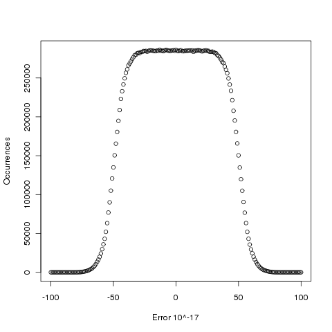
The results (raw data for R, Linux C and Cygwin C) show that around 5.6% of values are off by one in the last (15th) digit (Cygwin was slightly worse at 5.7%). The results for R/Linux C were almost identical and a quick check of the R source tree showed that R calls the C library function to evaluate log (it is a bit worrying that R is dependent on the host maths library, they should think about replacing this dependency by something like MPFR tout suite; even though the 64-bit glibc library is of very high quality it still has an environmental dependency).
Being off by one in the last decimal place is unlikely to keep many people awake at night. But if we want a measure of quality, is percentage of inaccurate values a useful measure of math library quality? Provided it is coupled with the amount of inaccuracy, I think this is a useful measure.
Recent Comments