Archive
After 55.5 years the Fortran Specialist Group has a new home
In the 1960s and 1970s, new developments in Cobol and Fortran language standards and implementations regularly appeared on the front page of the weekly computer papers (Algol 60 news sometimes appeared). Various language user groups were created, which produced newsletters and held meetups (this term did not become common until a decade or two ago).
In January 1970 the British Computer Society‘s Fortran Specialist Group (FSG) held its first meeting and 55.5 years later (this month) this group has moved to a new parent organization the Society of Research Software Engineering. The FSG is distinct from BSI‘s Fortran Standards panel and the ISO Fortran working group, although they share a few members.
I believe that the FSG is the oldest continuously running language user group. Second place probably goes to the ACCU (Association on C and C++ Users) which was started in the late 1980s. Like me, both of these groups are based in the UK (the ACCU has offshoots in other countries). I welcome corrections from readers familiar with the language groups in other countries (there were many Pascal user groups created in the 1980s, but I don’t know of any that are still active). COBOL is a business language, and I have never seen a non-vendor meetup group that got involved with language issues.
The plot below shows estimated FSG membership numbers for various years, averaging 180 (thanks to David Muxworthy for the data; code+data):

My experience of national user groups is that membership tends to hover around a thousand. Perhaps the more serious, professional approach of the BCS deters the more casual members that haunt other user groups (whose membership fees help keep things afloat).
What are the characteristics of this Fortran group that have given it such a long and continuous life?
- It was started early. Fortran was one of the first, of two (perhaps three), widely used programming languages,
- Fortran continued to evolve in response to customer demand, which made it very difficult for new languages to acquire a share of Fortran’s scientific/engineering market. Compiler vendors have kept up, or at least those selling to high-end power customers have (the Open source Fortran compilers have lagged well behind).
Most developers don’t get involved with calculations using floating-point values, and so are unfamiliar with the multitude of issues that can have a significant impact on program output, e.g., noticeably inaccurate results. The Fortran Standard’s committee has spent many years making it possible to write accurate, portable floating-point code.
A major aim of the 1999 revision of the C Standard was to make its support for floating-point programming comparable to Fortran, to entice Fortran developers to switch to C,
- people being willing to dedicate their time, over a long period, to support the activities of this group.
The minutes of all the meetings are available. The group met four times a year until 1993, and then once or twice a year. Extracting (imperfectly) the attendance from the minutes finds around 525540 unique names, with 322350 attending once and one person attending 8155 meetings. The plot below shows the number of people who attended a given number of meetings (code+data):

The survival of any group depends on those members who turn up regularly and help out. The plot below shows a sorted list of FSG member tenure, in years, excluding single attendance members (code+data):

Will the FSG live on for another 55 years at the Society of Research Software Engineering?
Fortran continues to be used in a wide range of scientific/engineering applications. There is a lot of Fortran source out there, but it’s not a fashionable language and so rarely a topic of developer conversation. A group only lives because some members invest their time to make things happen. We will have to wait and see if this transplanted groups attracts a few people willing to invest in it.
Update the next day. Added attendance from pdf minutes, and removed any middle initials to improve person matching.
Will incorrect answers be biased towards one arm of an if-statement?
Sometimes it is possible to deduce which arm of a nested if-statement will be executed by looking at the form of the conditional expression in the outer if-statement, as in:
if ((L < M) && (M < H)) if (L < H) ; // Execution always end up here else ; // dead code |
but not in:
if ((L > M) && (M < H)) if (L < H) ; // Could end up here else ; // or here |
I ran an experiment at the 2012 ACCU conference where subjects saw nested if-statements like those above and had to specify which arm of the nested if-statement would be executed.
Sometimes subjects gave an answer specifying one arm when in fact both arms are possible. Now dear reader, do you think these incorrect answers will specify the then arm 50% of the time and the else arm 50% or do you think that that incorrect answers will more often specify one particular arm?
Of course I should have thought about this before I started to analyse the data, but this question is unrelated to the subject of the experiment and has only just cropped up because of the unexpectedly high percentage of this kind of incorrect answer. I had an idea what the answer would be but did not stop and think about relative percentages, rushing off to write a few lines of code to print the actual totals, so now my mind is polluted by knowing the answer (well at least for one group of subjects in one experiment).
Why does this “one arm preference” issue matter? The Bayesians out there will insist that the expected distribution (the prior in Bayesian terminology) of incorrectly chosen arms be factored in to the calculation of the probability of getting the numbers seen in the results. The paper Belgian euro coins: 140 heads in 250 tosses – suspicious? gives a succinct summary of the possibilities.
So I have decided to appeal to my experienced readership, yes YOU!
For those questions where the actual execution cannot be predicted in advance, from knowledge of the relative values of variables appearing in the outer if-statement, when an incorrect answer is given should the analysis assume:
- a 50/50 split of incorrect answers between each arm, or
- subjects are more likely to pick one arm; please specify a percentage breakdown between arms.
No pressure, but the submission deadline is very late tomorrow.
The results from the whole experiment will get written up here in future posts.
Update (three days later): Nobody was willing to stick their head above the parapet 🙁
There were 69 correct answers and 16 incorrect answers to questions whose answer was “both arm”. Ten of those incorrect answers specified the ‘then’ arm and 6 the ‘else’; my gut feeling was that there should be even more ‘then’ answers. If there was no “first arm” there is an equal probability of a subject’s incorrect answer appearing in either arm; in this case the probability of a 10/6 split is 12% (so my gut feeling was just hunger pangs after all).
Descriptive statistics of some Agile feature characteristics
The purpose of software engineering research is to figure out how software development works so that the software industry can improve its quality/timeliness (i.e., lower costs and improved customer satisfaction). Research is hampered by the fact that companies are not usually willing to make public good quality data about the details of their software development processes.
In mid July a post on the ACCU general mailing list caught my eye and I followed a link to a very interesting report, went to visit 7digital a few weeks later, told them about my empirical software engineering with R book and how I wanted to make all the data I used available to readers and they agreed to make the data public! The data arrived at the start of August and I spent the rest of the month analyzing it (the R code I used to analyse it).
Below is a draft of what will eventually appear in the book. As always comments welcome, particularly if you can extract more information from the 7digital data (the mapping of material to WordPress blog format might still be flaky in places).
Agile feature characteristics
Traditionally software development projects work towards releasing product updates on prespecified dates, often with a release cycle of between once or twice a year and with many updates included in each release. In contrast to this approach development groups following an Agile method <book ???> make frequent releases with each containing a small incremental update (Agile is an umbrella term applied to a variety of iterative and incremental software development methodologies).
Rationale for the Agile approach includes getting rapid feedback from customers on the direction of developments and maximizing return on software investment by getting newly implemented features into customers hand almost immediately.
The large number of releases (compared to other approaches) has the potential to provide enough data for meaningful statistical analysis of questions such as how often new features are released and the number of features under development at any time.
7digital<book 7Digital_12> is a digital media delivery company that operates an international on-line digital music store (www.7digital.com) and provides business to business digital media services via an open API platform. At 7digital software development is done using an Agile process and since April 2009 various items of information have been recorded <book Bowley_12>; 7digital are open about there process and have made this information publicly available and it is analysed here.
Data
The data consists of information on the 3,238 features implemented by the 7digital team between April 2009 and July 2012; this information consists of three dates (Prioritised/Start Development/Done), a classification of the feature as one of nine possible internal types (i.e.,
During the recording period the number of developers grew from 14 to 35.
The start/done dates represent an elapsed time period, a wide variety of factors can cause work on the implementation of a feature to be stalled for a period of time, i.e., the time difference need not represent total development time.
The Agile process gives a great deal of flexibility to developers about which projects they chose to work on. Information on the number of developers working on the implementation of individual features was not recorded.
Is the data believable?
As discussed elsewhere [checking data quality] measurements involving people are likely to be subject more external influences than measurements of inanimate objects such as source code, they are also more difficult to replicate and are open to those being measured influencing the results in their favor.
The following is what is known about the 7digital measurement process.
The data recording was done by whoever ran the Agile stand-up session at the start of the day.
What unit of time measurement is appropriate for analysing an Agile process? While fine grained measurements are the ideal they have the potential to require nontrivial effort from those reporting the values, are open to individual interpretation (e.g., when exactly did work start/stop on this feature?) and subject to human error (e.g., forgetting to note the event when it happened and having to recall it later). The day was chosen as the basic unit of time measurement; in light of the time needed to implement most features this may seem too large, but this choice has the advantage of being the natural unit of measurement in that developers meet together every morning to discuss progress and that days work and being so broad makes it more likely that start/end times will be consistently applied as well as less prone to inaccurate recall later.
Goodhart’s law (it is really an observation of human behavior rather than a law) says “Any observed statistical regularity will tend to collapse once pressure is placed on it for control purposes.” If the measurements collected were actively used to control or evaluate the development team then the developers would be motivated to move the measurements in the direction that was favorable to them. 7digital do not attempt to use the measurements for control or evaluation or developers and developers have no motive change their behavior based on being measured.
I find the data believable in that the measurement process is not so expensive or cumbersome that developers are unwilling to attempt to report accurate data and not being directly effected by the results means they have no motive for changing their behavior to influence the measurements.
Believable data does not mean the data is error free. The following is a count of the days of the week on which feature implementations were recorded as being Done. Monday is day 0 and the counts for Saturday/Sunday should be zero; assuming that Friday/Monday had been intended the non-zero values suggest a 2-4% error rate, comparable with human error rates for low stress/non-critical work.
> table(Done.day[(Done.day <= 650)] %% 7) 0 1 2 3 4 5 6 227 225 214 243 177 8 7 > table(Done.day[(Done.day > 650)] %% 7) 0 1 2 3 4 5 6 443 483 455 473 270 4 9 |
Predictions made in advance
Your author is not aware of any empirically based theory of Agile feature development capable of making predictions about development time related questions.
The analysis described here is purely descriptive; there is no attempt to build predictive models or compare the data against any existing theory.
The results from this data analysis (and all analysis in this book) are to provide information that will help software developers do a better job. What information can be extracted that would be useful to 7digital? This has proved to be a something of a chicken-and-egg question because people are interested in seeing the results before deciding whether they are useful. The following issues are of general interest:
- characteristics of the time taken to implement new features,
- variations in the number of different kinds of features (e.g., bug/non-bug) over time,
Applicable techniques
Overview of data
The data consists of start/finish times for the implementations of features and the overview information that springs to mind is average number of features implementation starts per time interval and average time taken to implement a feature. The figure below is a good enough approximation to this information to get a rough idea of its characteristics (e.g., the effect of weekends and holidays have not been taken into account and a 30 day rolling mean has been applied to smooth out daily fluctuations).
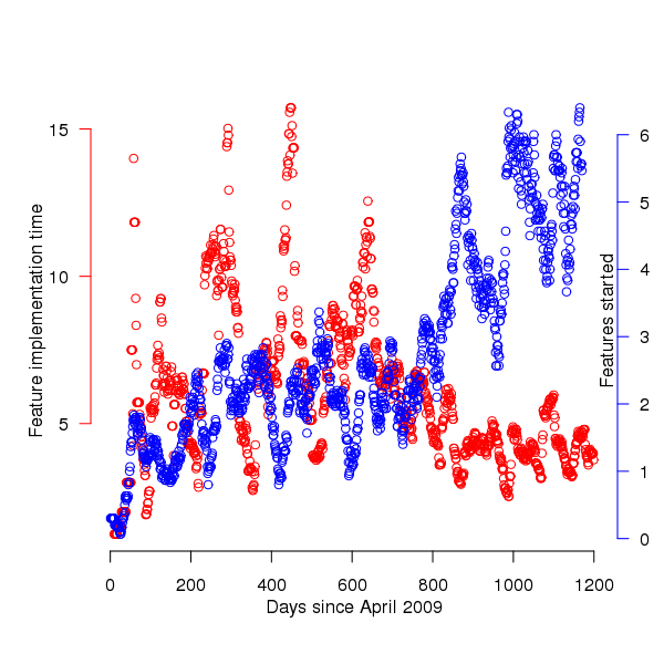
Figure 1. Average number of feature implementations started (blue) and their average duration (red); a 30 day rolling mean has been applied to both. Data courtesy of 7digital.
The plot appears to have two parts, before and after day 650 (or thereabouts). After day 650 the oscillations in feature implementation time die down substantially and the rate at which new feature implementations are started steadily increases. Possible reasons for the larger variations in the first 650 days include less expertise in organizing features into smaller work items and larger features being needed during the earlier stages of product development.
Obviously shorter implementation times make it possible to start work on more new features, however new feature starts continues to increase while implementation time stabilises around a lower value. Possible causes for the continuing increase in new feature starts include an increase in the number of developers and/or existing developers becoming more skilled in breaking work down into smaller features (i.e., feature implementation time stays about the same because fewer developers are working on each feature, making developers available to start on new features).
Software product development is a complicated business and a wide variety of different events and processes are likely to have contributed to the patterns of behavior seen in the data. While developers write the software it is customers who report most of the bugs and one of the goals of following an Agile methodology is rapid response to customer feedback (e.g., deciding which features need to be implemented and which left out). Customer information is not present in the dataset.
Are the same processes generating the apparent two phase behavior?
Any pattern of behavior is generated by a set of processes and when a pattern of behavior changes it is worthwhile asking how the processes driving the behavior changed.
Fitting a statistical distribution to a dataset is useful in that many distributions are known to be generated by processes having specified behaviors. Being able to fit the same distribution to both the pre and post 650 day datasets suggests that the phase change seen was not a fundamental change but akin to turning the volume knob of the distribution parameters one way or the other. If the datasets are best fitted by different distributions then the processes generating the two patterns of behavior are potentially very different.
Of the two characteristics plotted the feature implementation time appears to undergo the largest change of behavior and so the distribution of implementation times for the two phases is analysed here.
| Moment | Initial 650 days | After 650 days |
|---|---|---|
|
Median
|
3
|
3
|
|
Mean
|
7.6
|
4.6
|
|
Variance
|
116.4
|
35.0
|
|
Skewness
|
3.3
|
4.9
|
|
Kurtosis
|
19.2
|
30.4
|
A quick look at the data shows that many features are implemented in a single day and only a few take more than a week, one distribution having this pattern of behavior is the power-law. The table above shows that the variance is much larger than the mean and the distribution has a large positive skew, properties shared by the [negative binomial distribution]. The figure below is a plot of the number of features requiring a given number of elapsed working days for their implementation (top first 650 days, all features finished after 650 days), along with two power-law and a negative binomial distribution fit to the data.
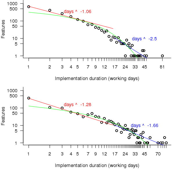
Figure 2. Number of features whose implementation took a given number of elapsed workdays. Top first 650 days, bottom after 650 days. Green line is the fitted negative binomial distribution. Data courtesy of 7digital.
The power-law fits were obtained by splitting the data into two parts, shorter/longer than 16 days (after noticing that visually the combined dataset seemed to have this form, less noticeable in the two subsets) and performing nonlinear regression using nls to find good fits for the parameters a and b (whose initial starting values converged without needing manual tuning).
pow_equ=nls(num.features ~ a*days^b, start=list(a=1200, b =-2)) y=predict(pow_equ, days) lines(days, y) |
While the power-law fits are not very good overall one of them does provide an easy to remember seat of the pants method for approximating the probability of a project taking a small number of days to complete (e.g., for  it is
it is 
[sum(1/(1:16)) is 3.38]). The approximation is also a reasonable fit for subsets of the features (e.g., different kinds of bugs).
The R package fitdistrplus contains functions for matching and fitting a dataset against known commonly occurring distribution. The Cullen and Frey graph produced by a call to descdist suggests that a negative binomial distribution is the best fitting of those tested (agreeing with the ad-hoc conclusion jumped to above).
descdist(p\$Cycle.Time, discrete=TRUE, boot=100) |
The function fitdist returns values for the parameters providing the appropriate fit to the specified dataset and distribution.
fd=fitdist(p\$Cycle.Time, "nbinom", method="mle") # Fit to a negative binomial distribution size.ct=fd\$estimate[1] mu.ct=fd\$estimate[2] # Plot distribution using fitted parameters plot(dnbinom(1:93, size=size.ct, mu=mu.ct)*length(p\$Cycle.Time), xlim=c(1,90), ylim=c(1,1200), log="xy") |
The figure above shows that the negative binomial distribution could be a reasonable fit if the percentage of single day features was not so high. Two possibilities spring to mind:
- the data does not include any counts for zero days which is one of the possible values supported by the negative binomial distribution (obviously feature implementations cannot take zero days),
- measurement quantization introduces significant uncertainty for shorter implementations, if the minimum unit of measurement were less than 1 day the fit might be much better because some feature implementations take half-a-day while others take a whole day.
It is possible to adjust the negative binomial equation to move the lower bound from zero to one. The package gamlss supports what is known as zero-truncation and the figure below shows the zero-truncated negative binomial distribution fitted to the pre/post 650 day counts.
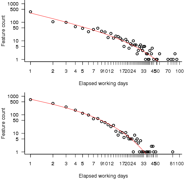
Figure 3. A zero-truncated negative binomial distribution fitted to the number of features whose implementation took a given number of elapsed workdays; top first 650 days, bottom after 650 days. Data courtesy of 7digital.
The quality of fit is much better for the pre 650 day data compared to the post 650 data.
> qual.pre650 AIC log.likelihood 6109.225 -3052.612 > qual.post650 AIC log.likelihood 9923.509 -4959.754 |
Modifying the negative binomial distribution to handle a dataset not containing zeroes improves the fit, can the fit be further improved by adjusting for measurement quantization?
One possibility is to simulate measuring feature implementation in units smaller than a day; the following code multiplies the implementation time by two and randomly decides whether to subtract one, i.e., maps measurements made in days to a possible set of measurements made in half days.
num.features=length(cycle.time) dither=as.integer(runif(num.features, 0, 1) > 0.33) return(2*cycle.time-dither) |
Fitting 1,000 randomly modified half-day measurements and averaging over all results shows that the fit is slightly worse than the original data (as measured by various goodness of fit criteria):
> fit.quality(p\$Cycle.Time[Done.day < 650]) loglikelihood AIC BIC -3438.284 6880.567 6890.575 > rowMeans(replicate(1000, fit.quality(sub.divide(p\$Cycle.Time[Done.day < 650])))) loglikelihood AIC BIC -4072.721 8149.442 8159.450 |
As discussed in the section on [properties of distributions] the negative binomial distribution can be generated by a mixture of [Poisson distribution]s whose means have a [Gamma distribution]. There are other distributions that can be generated through a mixture of Poisson distributions, are any of them a better fit of the data? The Delaporte distribution <book ???> sometimes fits very slightly better and sometimes slightly worse (see chapter source code for details); the difference is not large enough to warrant switching from a relatively well known distribution to one that is rarely covered in text books or supported in software; if data from other projects is best fitted by a Delaporte distribution then a switch may well be worthwhile.
The data subset corresponding to p$Type == "Production Bug" fits significantly better than the complete dataset (i.e., AIC = 3729) while the fit for the subset p$Type == "MMF" is comparable to the complete dataset (i.e., AIC of 7251).
Both datsets appear to follow the same distribution, the negative binomial distribution (with zero-truncation), with the initial 650 days having a greater mean and variance than post 650 days. The Poisson distribution is often encountered in processes involving events in time and one can imagine it applying to the various processes involved in the implementation of a feature; why the means of these Poisson distributions might follow a Gamma distribution is harder to fathom and is left for another day (it implies that both the Poisson means are decreasing and that the variance of the means is decreasing)
Do any other equations fit the data? Given enough optional parameters it is always possible to find an equation that is a good fit to the data. The following call to nls shows that the equation  fits the complete dataset rather well.
exp_mod=nls(num.features ~ a*exp(b*days^c), start=list(a=10000, b=-2.0, c=0.4)) |
This equation is unappealing because of its lack of similarity with equations seen in many other areas of research, an exponential whose exponent has the form of  raised to a fractional power is rarely encountered. There is a great deal of uncertainty when analysing data for the first time and being able to fit a form of equation used by other researchers provides a big comfort factor.
How many new feature implementations are started on each day?
The table below give the probability of a given number of new feature implementations starting on any day. There are sufficient multi-day implementations that on almost 20% of days no new feature implementations are started. An exponential equation is the commonly encountered form that provides an approximate fit to these values (i.e.,  ).
).
| 0 | 1 | 2 | 3 | 4 | 5 | 6 | 7 | 8 | 9 |
|---|---|---|---|---|---|---|---|---|---|
|
0.18
|
0.12
|
0.15
|
0.1
|
0.099
|
0.081
|
0.076
|
0.043
|
0.033
|
0.029
|
Time dependent patterns in the data
7digital is a growing company and we would expect that the rate of creation of features would increase over time, also as the size of the code base and the customer base increases the rate at which bugs are accepted for fixing is likely to increase.
The number of features developments started per day is one way of comparing different types of features. Plotting this information (see top left) shows that there is a great deal of variation over very short periods of time. This variation can be smoothed using a [rolling mean] to bring out the trends (the rollmean function in package zoo); the other plots show 20, 50 and 120 day rolling means for bugs (red) and non-bugs (blue) and the non-bug/bug feature ratio (black).
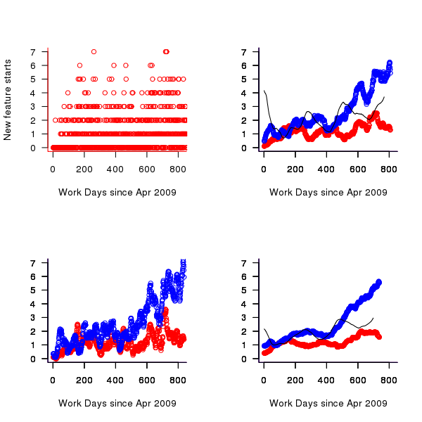
Figure 4. Number of feature developments started on a given work day (red bug fixes, blue non-bug work, black ratio of two values; 20 day rolling mean bottom left, 50 day top right, 120 day bottom right).
Both the number of bugs and non-bug features has trended upwards, as has the ratio between them. While it is tempting to suggest that this increase has been generated by the significant increase in number of developers over the time period, it is also possible the group has become better at dividing work into smaller feature work items or that having implemented the basic core of the products less work is now needed to create new features. The information present in the data is not sufficient to attempt to provide believable explanations for the upward trend.
Time series analysis
A preliminary data analysis technique for time data is to plot the current values against their lagged values for various lags. The output from the R function lag.plot for the number of in-progress features is shown below; apart from clustering the plots do not show any noticeable relationships in the data.
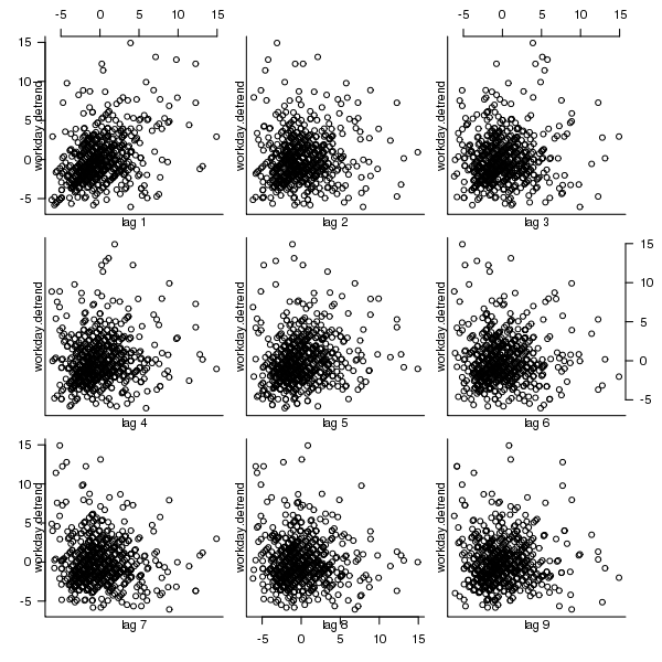
Figure 5. Scatterplot of number of features currently in-progress against various time lags (in working days).
Over longer timescales do the number of in-progress feature implementations have noticeable seasonal variations (e.g., greater in summer and Christmas/year year when developers are likely to be away)?
[Autocorrelation] is the cross-correlation of a time varying signal with itself, i.e., the correlation between a measurement occurring at time  and another one occurring at time
  ; changes in correlation as
  increases can be used to infer information about periodic changes over time.
The number of in-progress features appears to be increasing over time (top left of figure below) and this trend away from zero needs to be adjusted for before an autocorrelation is calculated. The feature implementation recording process did not happen over night and took a while before it covered all work performed; comparing a linear fit of all data (pink line of top left of figure below) and all data from January 2010 (red line) shows that this startup period does not significantly bias the growth trend. However, it is possible that patterns of behavior present in the total set of work items over a period are not reflected in the first 250 days of recording (roughly 180 working days) and so these are excluded from this particular analysis. From feature duration measurements we know that over 70% of features take longer than a day to implement, so the data contains a lot of serial dependence which may affect the accuracy of the results.
trend=lm(day.totals ~ time(day.totals)) plot(day.totals, xlab="Days since Apr 2009", ylab="Features in-progress") abline(trend) day.detrend=day.totals - predict(trend) # Subtract out any global trend |
The bottom left of the figure below shows the variation of in-progress features about the trend line. The top right shows the autocorrelation function for this plot, the regular spikes are caused by weekends (when no work took place). Removing weekends from the analysis results in the autocorrelation shown in the bottom right.
Apart from some correlation having a one day lag the autocorrelation drops to zero almost immediately followed by what appear to be small random spikes. These small spikes do not look important enough to follow up. A very similar pattern is seen in the autocorrelation of the two 650-day phases (the initial 650 days has a larger correlation for lags of 2-5 days). It is possible that a seasonal oscillation in feature work exists but is not seen because the data is so noisy (i.e., contains significant variation between adjacent days).
Summing daily values to create weekly totals, which of provides some smoothing, and performing the above analysis again produces essentially the same results.
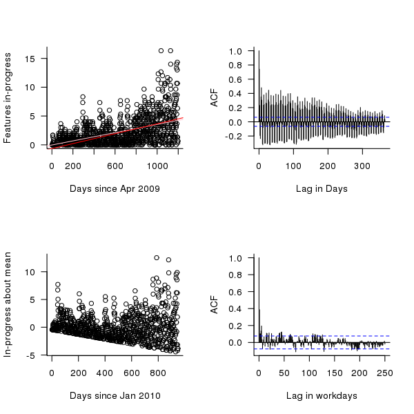
Figure 6. The number of features currently in-production on a given day since April 2009 (top left, pink line is a linear fit of all data, red line a linear fit of the data after day 250), the variation in this number about a linear trend line, excluding the first 250 days (bottom left), the autocorrelation function (top right) and the autocorrelation function with weekends removed from the data (bottom right).
Do reported bugs correlate with new feature releases?
When a feature is released the probability of a new bug being reported increases. Whether different bug probabilities should be assigned to bugfix releases and non-bugfix releases is discussed below. Based on this expectation we would expect to see a [cross correlation] between releases and number of bugs accepted for fixing. The more code a feature contains the more likely it is to contain a bug; however, no information on feature code size is provided so number of implementation work days is used as a measure of feature size.
The data does not specify which bugs belong to which features. It is to be expected that over time the probability of a bug being reported against a feature will decrease, reasons for this behavior include bugfixing, customers no longer using a feature and features being superseded by newer ones.
The figure below is the cross correlation between the ‘size’ of all features recorded as Done on a given day and all bugs recorded as Prioritised on a given date; the top plot is for all non-bugfix feature releases while the bottom plot is for all feature releases.
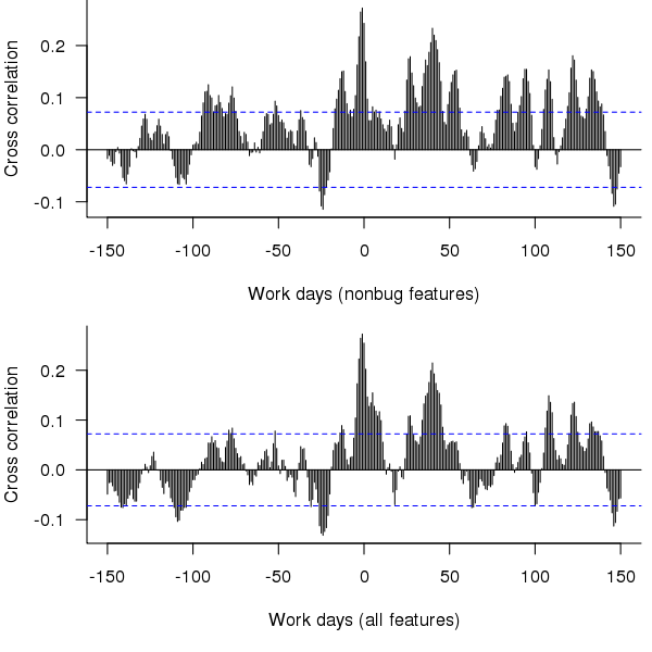
Figure 7. Cross correlation of feature release ‘size’ (top non-bugfix releases, bottom all releases) and date when bugs are prioritised.
The feature/bug cross correlation in the figure above should be zero for negative lags (i.e., no bugs can be reported for features that have not yet been released). One way of interpreting the pattern of correlation is that there some bugs are reported immediately after the release (perhaps by early adopters) followed by more bugs some 20 to 50 working days after release; other interpretations include there being a small amount of signal just visible behind lots of noise in the data or that the approximation used to estimate feature size is too crude.
Using weekly totals produces essentially the same result.
Summary of findings
The distribution of feature implementation times appears to follow a negative binomial distribution (with zero-truncation), with the values for the initial 650 days having a greater mean and variability (i.e., variance) than the following days.
There appears to be too much noise in the data for any time series signal involving mean values or a relationship between releases and bugs to be reliably extracted.
Acknowledgements
Thanks to 7digital for making the data available and being willing to make it public and to Rob Bowley for helping me to understand 7digital’s development environment.
Using identifier prefixes results in more developer errors
Human speech communication has to be processed in real time using a cpu with a very low clock rate (i.e., the human brain whose neurons fire at rates between 10-100 Hz). Biological evolution has mitigated the clock rate problem by producing a brain with parallel processing capabilities and cultural evolution has chipped in by organizing the information content of languages to take account of the brains strengths and weaknesses. Words provide a good example of the way information content can be structured to be handled by a very slow processor/memory system, e.g., 85% of English words start with a strong syllable (for more details search for initial in this detailed analysis of human word processing).
Given that the start of a word plays an important role as an information retrieval key we would expect the code reading performance of software developers to be affected by whether the identifiers they see all start with the same letter sequence or all started with different letter sequences. For instance, developers would be expected to make fewer errors or work quicker when reading the visually contiguous sequence consoleStr, startStr, memoryStr and lineStr, compared to say strConsole, strStart, strMemory and strLine.
An experiment I ran at the 2011 ACCU conference provided the first empirical evidence of the letter prefix effect that I am aware of. Subjects were asked to remember a list of four assignment statements, each having the form id=constant;, perform an unrelated task for a short period of time and then recall information about the previously seen constants (e.g., their value and which variable they were assigned to).
During recall subjects saw a list of five identifiers and one of the questions asked was which identifier was not in the previously seen list? When the list of identifiers started with different letters (e.g., cat, mat, hat, pat and bat) the error rate was 2.6% and when the identifiers all started with the same letter (e.g., pin, pat, pod, peg, and pen) the error rate was 5.9% (the standard deviation was 4.5% and 6.8% respectively, but ANOVA p-value was 0.038). Having identifiers share the same initial letter appears to double the error rate.
This looks like great news; empirical evidence of software developer behavior following the predictions of a model of human human speech/reading processing. A similar experiment was run in 2006, this asked subjects to remember a list of three assignment statements and they had to select the ‘not seen’ identifier from a list of four possibilities. An analysis of the results did not find any statistically significant difference in performance for the same/different first letter manipulation.
The 2011/2006 experiments throw up lots of questions, including: does the sharing a prefix only make a difference to performance when there are four or more identifiers, how does the error rate change as the number of identifiers increases, how does the error rate change as the number of letters in the identifier change, would the effect be seen for a list of three identifiers if there was a longer period between seeing the information and having to recall it, would the effect be greater if the shared prefix contained more than one letter?
Don’t expect answers to appear quickly. Experimenting using people as subjects is a slow, labour intensive process and software developers don’t always answer the question that you think they are answering. If anybody is interested in replicating the 2011 experiment the tools needed to generate the question sheets are available for download.
For many years I have strongly recommended that developers don’t prefix a set of identifiers sharing some attribute with a common letter sequence (its great to finally have some experimental backup, however small). If it is considered important that an attribute be visible in an identifiers spelling put it at the end of the identifier.
See you all at the ACCU conference tomorrow and don’t forget to bring a pen/pencil. I have only printed 40 experiment booklets, first come first served.
Randomizing a list of items using sort() and rand()
I’m busy putting together the experiment I will be running at the ACCU conference next week. If you are attending the conference please reserve your Thursday lunchtime slot for taking part as a subject!
Experiment generation invariably involves randomizing the sequence of items seen by every subject. While few languages support a randomise function many support sorting and random number generation. These two functions can be combined to create a randomize function; simply append a random number to the start of each item, sort it and then strip off the random number. Voilà a randomized list (awk code below).
function rand_items(items) { for (v in items) { items[v]=rand() " " items[v] } asort(items) for (v in items) { sp_pos=index(items[v], " ") items[v]=substr(items[v], sp_pos+1) } } |
This randomization problem is not yet listed on Rosetta code and probably has longer solutions in other languages.
Update (the next day).
The glow I have had for the last 10 years over coming up with a neat solution to a problem has now disappeared. Following the link kindly provided by D. Herring in the comments eventually lead me to the Fisher-Yates shuffle, which has ") performance (the call to sort is probably
performance (the call to sort is probably ") . The following shuffles a deck of cards:
. The following shuffles a deck of cards:
for (i = 0; i < 52; i++) { j = i + (rand() % (52 - i)); tmp = card[i]; card[i] = card[j]; card[j] = tmp; } |
The proof of the uniform shuffling behavior of Fisher-Yates (also known as Knuth shuffle) is straight forward but not nearly as appealing as using rand and sort.
The complexity of three assignment statements
Once I got into researching my book on C I was surprised at how few experiments had been run using professional software developers. I knew a number of people on the Association of C and C++ Users committee, in particular the then chair Francis Glassborow, and suggested that they ought to let me run an experiment at the 2003 ACCU conference. They agreed and I have been running an experiment every year since.
Before the 2003 conference I had never run an experiment that had people as subjects. I knew that if I wanted to obtain a meaningful result the number of factors that could vary had to be limited to as few as possible. I picked a topic which has probably been the subject of more experiments that any other topics, short term memory. The experimental design asked subjects to remember a list of three assignment statements (e.g., X = 5;), perform an unrelated task that was likely to occupy them for 10 seconds or so, and then recognize the variables they had previously seen within a list and recall the numeric value assigned to each variable.
I knew all about the factors that influenced memory performance for lists of words: word frequency, word-length, phonological similarity, how chunking was often used to help store/recall information and more. My variable names were carefully chosen to balance all of these effects and the information content of the three assignments required slightly more short term memory storage than subjects were likely to have.
The results showed none of the effects that I was expecting. Had I found evidence that a professional software developer’s brain really did operate differently than other peoples’ or was something wrong with my experiment? I tried again two years later (I ran a non-memory experiment the following year while I mulled over my failure) and this time a chance conversation with one of the subjects after the experiment uncovered one factor I had not controlled for.
Software developers are problem solvers (well at least the good ones are) and I had presented them with a problem; how to remember information that appeared to require more storage than available in their short term memories and accurately recall it shortly afterwards. The obvious solution was to reduce the amount of information that needed to be stored by simply remembering the first letter of every variable (which one of the effects I was controlling for had insured was unique) not the complete variable name.
I ran another experiment the following year and still did not obtain the expected results. What was I missing now? I don’t know and in 2008 I ran a non-memory based experiment. I still have no idea what techniques my subjects are using to remember information about three assignment statements that are preventing me getting the results I expect.
Perhaps those researchers out there that claim to understand the processes involved in comprehending a complete function definition can help me out by explaining the mental processes involved in remembering information about three assignment statements.
Finding the ‘minimum’ faulty program
A few weeks ago I received an inquiry about running a course/workshop on compiler writing. This does not does not happen very often and it reminded me that many years ago the ACCU asked if I would run a mentored group on compiler writing, I was busy writing a book at the time. The inquiry got me thinking it would be fun to run a compiler writing mentored group over a 6-9 month period and I emailed the general ACCU reflector asking if anybody was interested in joining such a group (any reader wanting to join the group has to be a member of the ACCU).
Over the weekend I had a brainwave for a project, automatic compiler test generation coupled with a program source code minimizer (I need a better name for this bit). Automatic test generation sounds great in theory but in practice whittling down the source code of those programs that result in a fault being exhibited, to create a usable sized test case that is practical for debugging purposes can be a major effort. What is needed is a tool to automatically do the whittling, i.e., a test case minimizer.
A simple algorithm for whittling down the source of a large test program is to continually throw away that half/third/quarter of the code that is not needed for the fault to manifest itself. A compiler project that took as input source code, removed half/third/quarter of the code and generated output that could be compiled and executed is realistic. The input/reduce/output process could be repeated until the generated source was considered to have reached some minima. Ok, this will soak up some cpu time, but computers are cheap and people are expensive.
Where does the test source code come from? Easy, it is generated from the same yacc grammar that the compiler, written by the mentored group member, uses to parse its input. Fortunately such a generation tool is available and ready to use.
The beauty is using the same grammar to generate tests and parse input. This means there is no need to worry about which language subset to use initially and support for additional language syntax can be added incrementally.
Experience shows that automatically generated test programs quickly uncover faults in production compilers, even when working with language subsets. Compiler implementors are loath to spend time cutting down a large program to find the statement/expression where the fault lies, this project will produce a tool that does the job for them.
So to recap, the mentored group is going to write one or more automatic source code generators that will be used to stress test compilers written by other people (e.g., gcc and Microsoft). Group members will also write their own compiler that reads in this automatically generated source code, throws some of it away and writes out syntactically/semantically correct source code. Various scripts will be be written to glue this all together.
Group members can pick the language they want to work with. The initial subset could just include supports for integer types, if-statements and binary operators.
If you had trouble making any sense all this, don’t join the group.
Recent Comments