Archive
Chinese research in software engineering
China and the Future of Science is the title of a recent article on the blog The Scholar’s Stage. In a series of posts the author, Tanner Greer, has been discussing how Chairman Xi and the Chinese central committee have reoriented the party towards a new goal. In 2026, the aim of China’s communist enterprise is to lead humanity through what they call “the next round of techno scientific revolution and industrial transformation.”.
The Chinese view is that: the first industrial revolution happened in Britain, which was the most powerful country of the 19th century; the second and third (computers) industrial revolutions happened in the USA, which was the most powerful country of the 20th century; the fourth industrial revolution is going to happen in China, which is going to be the most powerful country of the 21st century.
This is a software engineering blog, so I will leave the discussion of any fourth industrial revolution and whether China will lead it to others.
One practical consequence of the Chinese central committee’s focus is lots of funding for science/engineering research, and Chinese academics incentivised to do world-class work. How do you measure an individual’s or institution’s research performance? The Chinese have adopted the Western metric, i.e., counting papers published (weighted by journal impact factor) and number of citations. In 2025, eight of the top ten universities in the CWTS Leiden Ranking are Chinese, with the top western university in the number three spot and the other appearing at number ten. In 2005, six of the top ten universities were in the US.
In a post reviewing software engineering in 2023, I said: “it was very noticeable that many of the authors of papers at major conferences had Asian names. I would say that, on average, papers with Asian author names were better than papers by authors with non-Asian names.”
If software engineering researchers in China are publishing highly cited papers, why am I not seeing blog posts discussing them or hearing people talk about them? The answer is the same for Chinese and Western papers, i.e., little or no industrial relevance (when I point this out to academics they tell me that their work will be found to be relevant in years to come; ha ha {at least in software engineering}).
I label much of the research in software engineering as butterfly-collecting, in the sense that project source code is collected (often via GitHub) and various characteristics are measured and discussed. Much like the biological world was studied 200 years ago. There is no over arching theory, or attempt to model the relationships between different collections.
The incentives have pushed Chinese researchers, in software engineering, to become better butterfly collectors than Western researchers. Also, like Western researchers, they are mostly analysing the data using pre-computer statistical techniques.
If the aim is to publish papers and attract citations, it makes sense for Chinese researchers to study the same topics as Western researchers and analyse the data using the same (pre-computer) statistical techniques. Papers are more likely to be accepted for publication by Westerner reviewers when the subject matter is familiar to those reviewers. There are many tales of researchers having problems publishing papers that introduce new ideas and techniques.
The Central committee don’t just want to appear to be leading the world in engineering research, they want the Chinese to be making the discoveries that enable China to be the most powerful country in the world. For software engineering this means some Chinese researchers must stop following the research agenda set by their Western counterparts, and start asking “what are the important problems in software engineering“, and then researching those problems. If they are effective, a few will be enough.
My Evidence-based Software Engineering book lists and organises some of possible questions to ask, and also contains examples of modern statistical analysis.
China has lots of very good researchers. Perhaps they have all been sucked into the mania vortex around LLMs, and we will have to wait for things to subside. Remember, major discoveries are often made by small group of people.
70% of new software engineering papers on arXiv are LLM related
Subjectively, it feels like LLMs dominate the software engineering research agenda. Are most researchers essentially studying “Using LLMs to do …”? What does the data on papers published since 2022, when LLMs publicly appeared, have to say?
There is usually a year or two delay between doing the research work and the paper describing the work appearing in a peer reviewed conference/journal. Sometimes the researcher loses interest and no paper appears.
Preprint servers offer a fast track to publication. A researcher uploads a paper, and it appears the next day, with a peer reviewed version appearing sometime later (or not at all). Preprint publication data provides the closest approximation to real-time tracking of research topics. arXiv is the major open-access archive for research papers in computing, physics, mathematics and various engineering fields. The software engineering subcategory is cs.SE; every weekday I read the abstracts of the papers that have been uploaded, looking for a ‘gold dust’ paper.
The python package arxivscraper uses the arXiv api to retrieve metadata associated with papers published on the site. A surprisingly short program extracted the 15,899 papers published in the cs.SE subcategory since 1st January 2022.
A paper’s titles had to capture people’s attention using a handful of words. Putting the name of a new tool/concept in the title is likely to attract attention. The three words in the phrase Large Language Model consume a lot of title space, but during startup the abbreviated form (i.e., LLM) may not be generally recognised. The plot below shows the percentage of papers published each month whose title (case-insensitive) is matched either the regular expression “llm” or “large language model” (code and data):

Peak Large Language Model appears to be at the end of 2024. As time goes by new phrases/abbreviations stop being new and attention is grabbed by other phrases. Did peak LLM in titles occur at the end of 2025?
A paper’s abstract summarises its contents and has space for a lot more words. The plot below shows the percentage of papers published each month whose abstract (case-insensitive) is matched by either the regular expression “llm” or “large language model” (code and data):
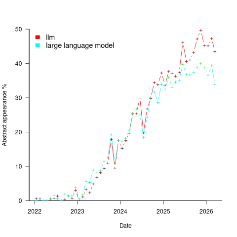
Peak, or plateauing, Large Language Model appears to be towards the end of 2025. Is the end of 2025 a peak of LLM in abstracts, or is it a plateauing with the decline yet to start? We should know by the end of this year.
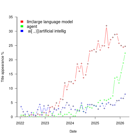
Other phrases associated with LLMs are AI, artificial intelligence and agents. The plot below shows the percentage of papers published each month whose title (case-insensitive) is matched by each of the regular expressions “llm|large language model“, or “ ai[ ,.)]|artificial intellig“, or “agent” (code and data):
Counting the papers containing one or more of these LLM-related phrases gives an estimate of the number of software engineering papers studying this topic. The plot below shows the percentage of papers published each month whose title or abstract (case-insensitive) is matched by one or more of the regular expressions “llm|large language model“, or “ ai[ ,.)]|artificial intellig“, or “agent” (code and data):
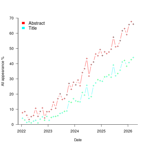
If the rate of growth is unchanged, around 18-month from now 100% of papers published in arXiv’s cs.SE subcategory will be LLM-related.
I expect the rate of growth to slow, and think it will stop before reaching 100% (I was expecting it to be higher than 70% in February). How much higher will it get? No idea, but herd mentality is a powerful force. Perhaps OpenAI going bankrupt will bring researchers to their senses.
Update
Martin Monperrus did an agentic replication of the analysis discussed in this post!
Identifier names chosen to hold the same information
Identifier naming is a contentious issue dominated by opinions and existing habits, with almost no experimental evidence (rather like software engineering practices in general).
One study found that around 40% of all non-white-space characters in the visible source of C programs are identifiers (comments representing 31% of the characters in the .c files), representing 29% of the visible tokens in the .c files.
Some years ago I spent a long time studying the word related experiments run by psychologists, looking for possible parallels with identifier usage. The crucial identifier naming factor is the semantic associations a name triggers in the reader’s mind. Choosing a name requires making a cost-benefit tradeoff. The greater quantity of information that might be communicated by longer names has to be balanced against both the cost of reading the name and ignoring the name when searching for other information.
The semantic association network present in a person’s head is the result of the words they have encountered and the context in which they were encountered. Different people are likely to make different associations. Shared culture and experiences increases the likelihood of shared naming associations.
A study by Nelson, McEvoy, and Schreiber gave subjects (over time, 6,000 students at the University of South Florida) a booklet containing 100 words, and asked them to write down the first word that came to mind that was meaningfully related or strongly associated to each of these words (data here, a total of 612,627 responses to 5,024 distinct words). The mean number of different responses to the same word was 14.4, with a standard deviation of 5.2.
There are patterns in the names of identifiers. For instance, operands of bitwise and logical operators have names that include words whose semantics is associated with the operations usually performed by these operands, such as: flag, status, state, and mask. One experiment (with a small sample size) found that developers make use of operand names to make operator precedence decisions.
A study by Feitelson, Mizrahi, Noy, Shabat, Eliyahu, and Sheffer, investigated the variable names chosen by developers to hold specific information. The 334 subjects (students and professional developers) were asked to suggest a name for a variable, constant, or data structure based on a description of the information it would contain, plus other questions relating to interpreting the semantics associated with a name.
The authors cite a problem that I think is actually a benefit: “A major problem in studying spontaneous naming is that the description of the context and the question itself necessarily use words.” When writing code a well-chosen name communications information about the context, which helps readers understand what is going on. The authors’ solution to this perceived problem was to give the description in either Hebrew or English (the subjects were native Hebrew speakers who are fluent in English), with subjects providing the name in English.
The answers to the 21 name generation questions had a mean of 53 distinct names (standard deviation 20.2; code and data). The table below shows the names chosen and the number of subjects choosing that name after seeing the description in Hebrew or English, for one of the questions.
Name Hebrew English b_elevator_door_state 1 b_is_door_open 1 curr_state 2 current_doors_state 1 door 3 1 door_current_status 1 door_is_closed 1 door_is_open 1 door_open 3 door_stat 1 door_state 10 12 door_status 4 doorstate 1 1 elevator_door_state 1 1 elevator_state 1 is_closed 1 1 is_door_closed 2 1 is_door_open 11 3 is_door_opened 2 2 is_elevator_open 1 is_o_pen 1 is_open 7 5 is_opened 2 state 1 status 1 status_of_door 1 |
While the names are distinct, some only differ by a permutation of words, e.g., door_is_open and is_door_open, or with one word missing, e.g., door_open and is_open, or two words missing, e.g., door.
If subjects are influenced by the description (e.g., using the word ordering that appears in the description, or only words from the description), the number of unique names would be smaller than if there was no such influence. The impact of influence would be that subjects seeing the English descriptions are likely to produce fewer unique names.
In 13 out of 21 questions, Hebrew subjects produced more unique names. However, a bootstrap test shows that the difference is not statistically significant.
I think a big threat to the validity of the study is only having subjects create one name. Writing software involves creating names for many variables, which has different cost-benefit tradeoffs than when creating a single variable. The names within a program share a common context and developers tend to follow informal patterns so that naming within the code has some degree of consistency. Adhering to these patterns restricts the possible set of names that might be chosen. Also, the existing use of a name may prevent it being reused for a new variable.
Programming competitions are one source for variable names implementing the same specification, at least for short program. Longer programs are more likely to have some variation in the algorithms used to implement the same functionality.
I expect greater consistency of identifier name selection within an LLM than across developers. LLM training will direct them down existing common patterns of usage, plus some random component.
Analysis of some C/C++ source file characteristics
Source code is contained in files within a file-system. However, source files as an entity are very rarely studied. The largest structural source code entities commonly studied are functions/methods/classes, which are stored within files.
To some extent this lack of research is understandable. In object-oriented languages one class per file appears to be a natural fit, at least for C++ and Java (I have not looked at other OO languages). In non-OO languages the clustering of functions/procedures/subroutines within a file appears to be one of developer convenience, or happenstance. Functions that are created/worked on together are in the same file because, I assume, this is the path of least resistance. At some future time functions may be moved to another file, or files split into smaller files.
What patterns are there in the way that files are organised within directories and subdirectories? Some developers keep everything within a single directory, while others cluster files by perceived functionality into various subdirectories. Program size is a factor here. Lots of subdirectories appears somewhat bureaucratic for small projects, and no subdirectories would be chaotic for large projects.
In general, there was little understanding of how files were typically organised, by users, within file-systems until around late 2000. Benchmarking of file-system performance was based on copies of the files/directories of a few shared file-systems. A 2009 paper uncovered the common usage patterns needed for generating realistic file-systems for benchmarking.
The following analysis investigates patterns in the source files and their contained functions in C/C++ programs. The information was extracted from 426 GitHub projects using CodeQL.
The 426 repos contained 116,169 C/C++ source files, which contained 29,721,070 function definitions. Which files contained C source and which C++? File name suffix provides a close approximation. The table below lists the top-10 suffixes:
   Suffix   Occurrences   Percent
     .c        53,931       46.4
     .cpp      49,621       42.7
     .cc        7,699        6.6
     .cxx       2,616        2.3
     .I           965        0.8
     .inl         403        0.3
     .ipp         400        0.3
     .inc         159        0.1
     .c++         136        0.1
.ic 128 0.1 |
CodeQL analysis can provide linkage information, i.e., whether a function is defined with C linkage. I used this information to distinguish C from C++ source because it is simpler than deciding which suffix is most likely to correspond to which language. It produced 56,002 files classified as containing C source.
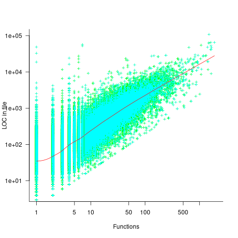
The full path to around 9% of files includes a subdirectory whose name is test/, tests/, or testcases/. Based on the (perhaps incorrect) belief that the characteristics of test files are different from source files, files contained under such directories were labelled test files. The plot below shows the number of files containing a given number of function definitions, with fitted power laws over two ranges (code and data):
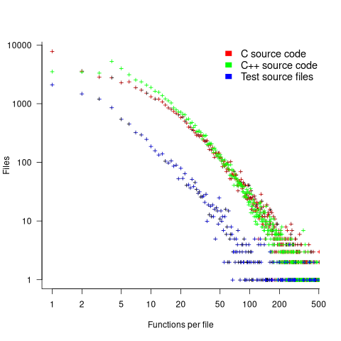
The shape of the file/function distribution is very surprising. I had not expected the majority of C files to contain a single function. For C++ there are two regions, with roughly the same number of files containing 1, 2, or 3 functions, and a smooth decline for files containing four or more methods (presumably most of these are contained in a class).
For C, C++ and test files, a power law could be fitted over a range of functions-per-file, e.g., between 6 and 2 for C, or between 4 and 2 for C++, or between 20 and 100 for C/C++, or 3 and more for test files. However, I have a suspicion that there is a currently unknown (to me) factor that needs to be adjusted for. Alternatively, I will get over my surprise at the shape of this distribution (files in general have a lognormal size, in bytes, distribution).
For C, C++ and test files, a power law is fitted over a range of functions-per-file, e.g., between 6 and 21 (exponent -1.1), and 22 and 100 (exponent -2) for C, between 4 and 21 (exponent -1.2), and 22 and 100 (exponent -2.2) for C++, between 4 and 50 (exponent -1.7), for test files. Files in general have a lognormal size, in bytes, distribution.
Perhaps a file contains only a few functions when these functions are very long. The plot below shows lines of code contained in files containing a given number of function, with fitted loess regression line in red (code and data):
A fitted regression model has the form  . The number of LOC per function in a file does slowly decrease as the number of functions increases, but the impact is not that large.
How are source files distributed across subdirectories? The plot below shows number of C/C++ files appearing within a subdirectory of a given depth, with fitted Poisson distribution (code and data):
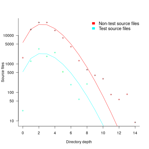
Studies of general file-systems found that number of files at a given subdirectory depth has a Poisson distribution with mean around 6.5. The mean depth for these C/C++ source files is 2.9.
Is this pattern of source file use specific to C/C++, or does it also occur in Java and Python? A question for another post.
Relative performance of computers since the 1990s
What was the range of performance of desktop’ish computers introduced since the 1990s, and what was the annual rate of performance increase (answers for earlier computers)?
Microcomputers based on Intel’s x86 family was decimating most non-niche cpu families by the early 1990s. During this cpu transition a shift to a new benchmark suite followed a few years behind. The SPEC cpu benchmark originated in 1989, followed by a 1992 update, with the 1995 update becoming widely used. Pre-1995 results don’t appear on the SPEC website: “Because SPEC’s processes were paper-based and not electronic back when SPEC CPU 92 was the current benchmark, SPEC does not have any electronic storage of these benchmark results.” Thanks to various groups, some SPEC89/92 results are still available.
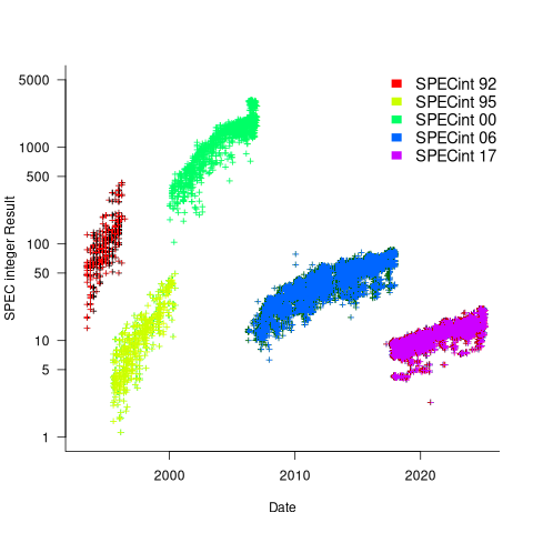
The following analysis uses the results from the SPEC integer benchmarks, which was changed in 1992, 1995, 2000, 2008, and 2017.
Every time a benchmark is changed, the reported results for the same computer change, perhaps by a lot. The plot below shows the results for each version of the benchmark (code+data):
Provide a few conditions are met, it is possible to normalise each set of results, allowing comparisons to be made across benchmark changes. First, results from running, say, both SPEC92 and SPEC95 on some set of computer needs to be available. These paired results can be used to build a model that maps result values from one benchmark to the other. The accuracy of the mapping will depend on there being a consistent pattern of change, i.e., a strong correlation between benchmark results.
The plot below shows the normalised results, along with regression models fitted to each release (code+data):
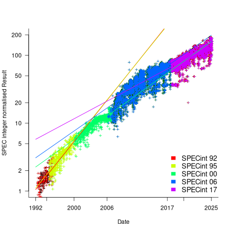
What happened around 2007? Dennard scaling stopped, and there is an obvious meeting of two curves as one epoch transitioned into another. Since 2007 performance improvements have been driven by faster memory, larger caches, and for some applications multiple on-die cpus.
The table below shows the annual growth in SPECint performance for each of the benchmark start years, over their lifetime.
      Year   Annual growth
      1992       26.2%
      1995       25.9%
      2000       14.2%
      2007       13.9%
2017 10.5% |
In 2025, the cpu integer performance of the average desktop system is over 100 times faster than the average 1992 desktop system. With the first factor of 10 improvement in the first 10 years, and the second factor of 10 in the previous 20 years.
Investigating an LLM generated C compiler
Spending over $20,000 on API calls, a team at Anthropic plus an LLM (Claude Opus version 4.6) wrote a C compiler capable of compiling the Linux kernel and other programs to a variety of cpus. Has Anthropic commercialised monkeys typing on keyboards, or have they created an effective sheep herder?
First of all, does this compiler handle a non-trivial amount of the C language?
Having written a variety of industrial compiler front ends, optimizers, code generators and code analysers (which paid off the mortgage on my house), along with a book that analysed of the C Standard, sentence by sentence (download the pdf), I’m used to finding my way around compilers.
Claude’s C compiler source appears to be surprisingly well written/organised (based on a few hours reading of the code). My immediate thought was that this must be regurgitation of pieces from existing compilers. Searches for a selection of comments in the source failed to find any matches. Stylistically, the code is written by an entity that totally believes in using abstractions; functions call functions that call functions, that call …, eventually arriving at a leaf function that just assigns a value. Not at all like a human C compiler writer (well, apart from this one).
There are some oddities in an implementation of this (small) size. For instance, constant folding includes support for floating-point literals. Use of floating-point is uncommon, and opportunities to fold literals rare. Perhaps this support was included because, well, an LLM did the work. But it increases the amount of code that can be incorrect, for little benefit. When writing a compiler in an implementation language different from the one being compiled, differences between the two languages can have an impact. For instance, Claude C uses Rust’s 128-bit integer type during constant folding, despite this and most other C compilers only supporting at most 64-bit integer types.
A README appears in each of the 32 source directories, giving a detailed overview of the design and implementation of the activities performed by the code. The average length is 560 lines. These READMEs look like edited versions of the prompts used.
To get a sense of how the compiler handled rarely used language features and corner cases, I fed it examples from my book (code). The Complex floating point type is supported, along with Universal Character Names, fiddly scoping rules, and preprocessor oddities. This compiler is certainly non-trivial.
The compiler’s major blind spot is failing to detect many semantic constraints, e.g., performing arithmetic on variables having a struct type, or multiple declarations of functions and variables with the same name in the same scope (the parser README says “No type checking during parsing”; no type checking would be more accurate). The training data is source code that compiles to machine code, i.e., does not contain any semantic errors that a compiler is required to flag. It’s not surprising that Claude C fails to detect many semantic errors. There is a freely available collection of tests for the 80 constraint clauses in the C Standard that can be integrated into the Claude C compiler test suite, including the prompts used to generate the tests.
A compiler is an information conveyor belt. Source is first split into tokens (based on language specific rules), which are parsed to build a tree representation and a symbol table, which is then converted to SSA form so that a sequence of established algorithms can be used to lower the level of abstraction and detect common optimizations patterns, the low-level representation is mapped to machine code, and written to a file in the format for an executable program.
The prompts used to orchestrate the information processing conveyor belt have not been released. I’m guessing that the human team prompted the LLM with a detailed specification of the interfaces between each phase of the compiler.
The compiler is implemented in Rust, the currently fashionable language, and the obvious choice for its PR value. The 106K of source is spread across 351 files (average 531 LOC), and built in 17.5 seconds on my system.
LLMs make mistakes, with coding benchmark success rates being at best around 90%. Based on these numbers, the likelihood of 351 files being correctly generated, at the same time, is  (with 99% probability of correctness we get
  ). Splitting the compiler into, say, 32 phases each in a directory containing 11 files, and generating and testing each phase independently significantly increases the probability of success (or alternatively, significantly reduces the number of repetitions of the generate code and test process). The success probability of each phase is:
  , and if the same phase is generated 13 times, i.e.,
 }/{log(1-0.90^{11})}") , there is a 99% probability that at least one of them is correct.
, there is a 99% probability that at least one of them is correct.
Some code need not do anything other than pass on the flow of information unchanged. For instance, code to perform the optimization common subexpression elimination does exist, but the optimization is not performed (based on looking at the machine code generated for a few tests; see codegen.c). Detecting non-functional code could require more prompting skill than generating the code. The prompt to implementation this optimization (e.g., write Rust code to perform value numbering) is very different from the prompt to write code containing common subexpressions, compile to machine code and check that the optimization is performed.
There is little commenting in the source for the lexer, parser, and machine code generators, i.e., the immediate front end and final back end. There is a fair amount of detailed commenting in source of the intervening phases.
The phases with little commenting are those which require lots of very specific, detailed information that is not often covered in books and papers. I suspect that the prompts for this code contains lots of detailed templates for tokenizing the source, building a tree, and at the back end how to map SSA nodes to specific instruction sequences.
The intermediate phases have more publicly available information that can be referenced in prompts, such as book chapters and particular papers. These prompts would need to be detailed instructions on how to annotate/transform the tree/SSA conveyed from earlier phases.
Algorithm complexity and implementation LOC
As computer functionality increases, it becomes easier to write programs to handle more complicated problems which require more computing resources; also, the low-hanging fruit has been picked and researchers need to move on. In some cases, the complexity of existing problems continues to increase.
The Linux kernel is an example of a solution to a problem that continues to increase in complexity, as measured by the number of lines of code.
The distribution of problem complexities will vary across application domains. Treating program size as a proxy for problem complexity is more believable when applied to one narrow application domain.
Since 1960, the journal Transactions on Mathematical Software has been making available the source code of implementations of the algorithms provided with the papers it publishes (before the early 1970s they were known as the Collected Algorithms of the ACM, and included more general algorithms). The plot below shows the number of lines of code in the source of the 893 published implementations over time, with fitted regression lines, in black, of the form  before 1994-1-1, and
  after that date (black dashed line is a LOESS regression model; code+data).
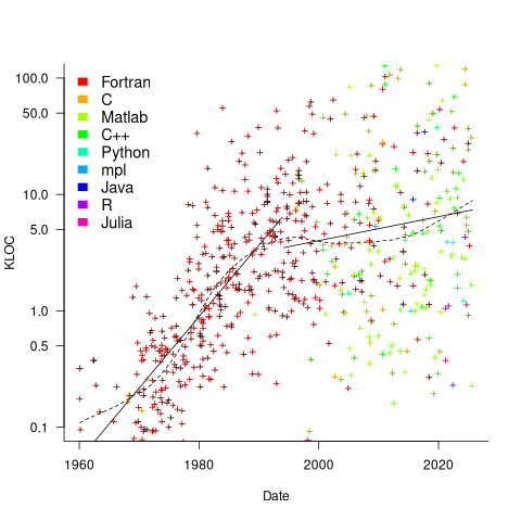
The two immediately obvious patterns are the sharp drop in the average rate of growth since the early 1990s (from 15% per year to 2% per year), and the dominance of Fortran until the early 2000s.
The growth in average implementation LOC might be caused by algorithms becoming more complicated, or because increasing computing resources meant that more code could be produced with the same amount of researcher effort, or another reason, or some combination. After around 2000, there is a significant increase in the variance in the size of implementations. I’m assuming that this is because some researchers focus on niche algorithms, while others continue to work on complicated algorithms.
An aim of Halstead’s early metric work was to create a measure of algorithm complexity.
If LLMs really do make researchers more productive, then in future years LOC growth rate should increase as more complicated problems are studied, or perhaps because LLMs generate more verbose code.
The table below shows the primary implementation language of the algorithm implementations:
  Language   Implementations
   Fortran        465
         C         79
    Matlab         72
       C++         24
    Python          7
         R          4
      Java          3
     Julia          2
MPL 1 |
If algorithms are becoming more complicated, then the papers describing/analysing them are likely to contain more pages. The plot below shows the number of pages in the published papers over time, with fitted regression line of the form  (0.38 pages per year; red dashed line is a LOESS regression model; code+data).
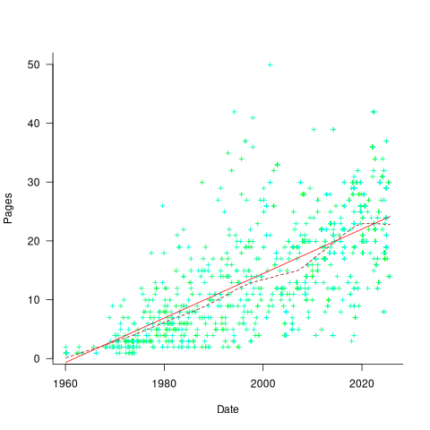
Unlike the growth of implementation LOC, there is no break-point in the linear growth of page count. Yes, page count is influence by factors such as long papers being less likely to be accepted, and being able to omit details by citing prior research.
It would be a waste of time to suggest more patterns of behavior without looking at a larger sample papers and their implementations (I have only looked at a handful).
When the source was distributed in several formats, the original one was used. Some algorithms came with build systems that included tests, examples and tutorials. The contents of the directories: CALGO_CD, drivers, demo, tutorial, bench, test, examples, doc were not counted.
Dennard scaling a necessary condition for Moore’s law
Dennard scaling was a necessary, but not sufficient, condition for Moore’s law to play out over many decades. Transistors generate heat, and continually adding more transistors to a device will eventually cause it to melt, because the generated heat cannot be removed fast enough. However, if the fabrication of transistors on the surface of a monolithic silicon semiconductor follows the Dennard scaling rules, then more, smaller transistors can be added without any increase in heat generated per unit area. These scaling rules were first given in the 1974 paper Design of Ion-Implanted MOSFET’S with Very Small Physical Dimensions by Dennard, Gaensslen, Hwa-Nien, Rideout, Bassous, and LeBlanc.
The plot below shows a vertical slice through a Metal–Oxide–Semiconductor Field-Effect Transistor (the kind of transistor used to build microprocessors), with the fabrication parameters applicable to Dennard scaling labelled. A transistor has three connections (only one is show), to the Source, the Drain, and the Gate. The Source and Drain are doped with an element from Group V to produce a surplus of electrons, while the substrate is doped with an element from Group III to create holes that accept electrons. A voltage applied to the Gate creates an electric field that modifies the shape of the depletion region (area above blue dashed line), enabling the flow of electrons between the Source and Drain to be switched on or off.
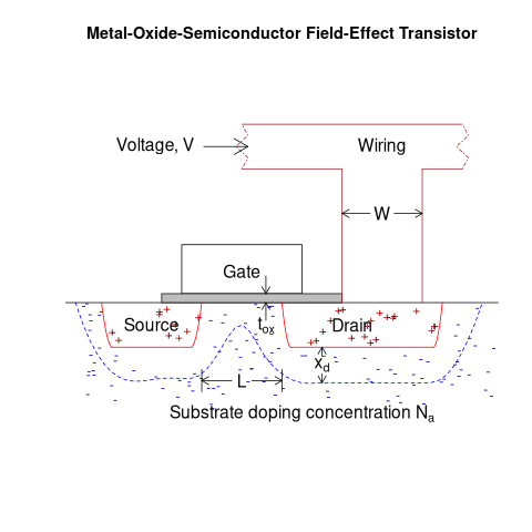
The parameters are: operating voltage,  , width of the connecting wires,
  , length of the channel between the Source and Drain,
  , thickness of the dielectric material (e.g., silicon oxynitride) under the Gate (shown in grey),
  , doping concentration,
  , and length of the depletion region,
  .
.
The power,  , consumed by any electronic device is
  , where
  is the current through it and the voltage across it. In an ideal transistor, in the off state
  and no power is consumed, and in the on state is at its maximum, but
  and no power is consumed. Power is only consumed during the transition between the two states, when both and are non-zero. In real transistors, there is some amount of leakage in the off/on states and a small amount of power is consumed.
Increasing the frequency,  , at which a transistor is operated increases the number of state transitions, which increases the power consumed. The power consumed per unit time by a transistor is
  . If there are
  transistors per unit area, the power consumed within that area is:
  .
.
The current, , can be written in terms of the factors that control it, as:  .
.
If the values of , , , and are all reduced by a factor of  (often around 30%, giving
  ), then
  is reduced by a factor of
  ,
, ^2=2") .
.
^2}}/{{L/alpha}*{t_{ox}/alpha}}}{V/alpha}={{N*f}/alpha^2}{{W*V^3}/{L*t_{ox}}}")
The area occupied by a transistor,  , decreases by , making it possible to increase the number of transistors within the same unit area to:
  . The transistors consume less power, but there are more of them, and power per unit area after the size reduction is the same as before reduction,
  .
.
Reducing the channel length, , has a detrimental impact on device performance. However, this can be overcome by increasing the density of the doping in the substrate, , by .
The maximum frequency at which a transistor can be operated is limited by its capacitance. The Gate capacitance is the major factor, and this decreases in proportion to the device dimensions, i.e., . A decrease in capacitance enables the operating frequency, , to increase. Capacitance was not included in the previous formula for power consumption. An alternative derivation finds that  , where
  is the capacitance, i.e., power consumption is unchanged when a frequency increase is matched by a corresponding decrease in capacitance.
The first working transistor was created in 1947 and the first MOSFET in 1959. The plot below, with data from various sources, shows the energy consumed by a transistor, fabricated in various years, switching between states, the red line is the fitted regression equation  , the green line is the fitted equation
  , and the grey line shows the Landauer limit for the energy consumption of a computation at room temperature (code and data; also see The End of Moore’s Law: A New Beginning for Information Technology by Theis and Wong):
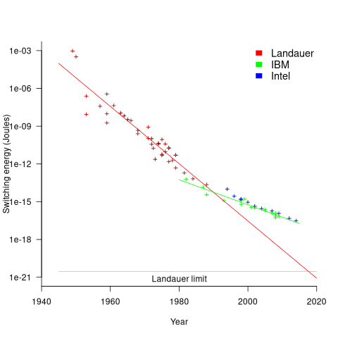
Scaling cannot go on forever. The two limits reached were voltage (difficulty reducing below 1V) and the thickness of the Gate dielectric layer (significant leakage current when less than 7 atoms thick).
The slow-down in the reduction of switching energy, in the plot above, is due to a slow-down in voltage reduction, i.e., reduction of less than .
In 2007, cpu clock frequency stopped increasing and Dennard scaling halted. In this year, the Gate and its dielectric was completely redesigned to use a high-k dielectric such as Hafnium oxide, which allowed transistor size to continue decreasing. However, since around 2014 the rate of decrease has slowed and process node numbers have become marketing values without any connection to the size of fabricated structures. Is 2014 the year that Moore’s law died? Some people think the year was 2010, while Intel still trumpet the law named after one of their founders.
Public documents/data on the internet sometimes disappears
People are often surprised when I tell them that documents/data regularly disappears from the internet. By disappear I mean: no links to websites hosting the data are returned by popular search engines, nothing on the Wayback Machine (including archive.org, which now has a Scholar page), and nothing on LLM suggested locations.
There is the drip-drip-drip of universities deleting the webpages they host of academics who leave the university (MIT is one of the few exceptions). Researchers often provide freely downloadable copies of their own papers via these pages, which may be the only free access (research papers are generally available behind a paywall). It’s great that the ACM has gone fully Open Access
Datasets that were once publicly available on government or corporate sites sometimes just disappear. Two ‘missing’ datasets I have written about are DACS dataset and Linux Counter data. This week, I found out that the detailed processor price lists that Intel used to publish are now disappeared from the web (one site hosts a dozen or so price lists; please let me know if you have any of these price lists).
I have lots of experience asking researchers for a copy of the data analysed in a paper they wrote, to be told something along the lines of “It’s on my old laptop”, i.e., disappeared.
It is to be expected that data from pre-digital times will only sometimes be available online. My interest in tracking the growth of digital storage has led to a search for details of annual sales of punched cards. I’m hoping that a GitHub repo of known data will attract more data.
The sites where researchers host the data analysed in their papers include (ordered in roughly the frequency I encounter them): GitHub, personal page, Zenodo, Figshare and the Center for Open Science.
Some journals offer a data hosting option for published papers. Access to this data can be problematic (e.g., agreeing to an overly restrictive license), or the link to the data might dead (one author I contacted was very irate that the journal was not hosting the data he had carefully curated, after they had assured him they were hosting it).
Research papers are connected by a web of citations. Being able to quickly find cited/citing papers makes it possible to do a much more thorough search of related work, compared to traditional manual methods. When it launched in 1997, CiteSeer was a revelation (it probably doubled the citations in my C book). Many non-computing papers could still only be found in university libraries, but by 2013 I no longer bothered visiting university libraries. ResearchGate launched in 2008, and in 2010 Semantic Scholar arrived. Unfortunately, the functionality of both CiteseerX and Semantic Scholar is a shadow of its former glory. ResearchGate continues to plod along, and Google Scholar has slowly gotten better and better, to become my paper search site of choice.
Keep a copy of your public documents/data on an Open access repository (e.g., GitHub, Zenodo, Figshare, etc). By all means make a copy available on your personal pages, but remember that these are likely to disappear.
Number of calls to/from functions vs function length
Depending on the language the largest unit of code is either a sequence of statements contained in a function/procedure/subroutine or a set of functions/methods contained in a larger unit, e.g., class/module/file. Connections between these largest units (e.g., calls to functions) provide a mechanism for analysing the structure of a program. These connections form a graph, and the structure is known as a call graph.
It is not always possible to build a completely accurate call graph by analysing a program’s source code (i.e., a static call graph) when the code makes use of function pointers. Uncertainty about which functions are called at certain points in the code is a problem for compiler writers wanting to do interprocedural flow analysis for code optimization, and static analysis tools looking for possible coding mistakes.
The following analysis investigates two patterns in the function call graph of C/C++ programs. While calls via function pointers can be very common at runtime, they are uncommon in the source. Function call information was extracted from 98 GitHub projects using CodeQL.
Functions that contain more code are likely to contain more function calls. The plot below shows lines of code against number of function calls for each of the 259,939 functions in whatever version of the Linux kernel is on GitHub today (25 Jan 2026), the red line is a regression fit showing  (the fit systematically deviates for larger functions {yet to find out why}; code and data):
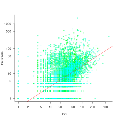
Researchers sometimes make a fuss of the fact that the number of calls per function is a power law, failing to note that this power law is a consequence of the number of lines per function being a power law (with an exponent of 2.8 for C, 2.7 for Java and 2.6 for Pharo). There are many small functions containing a few calls and a few large functions containing many calls.
Are more frequently called functions smaller (perhaps because they perform a simple operation that often needs to be done)? Widely used functionality is often placed in the same source file, and is usually called from functions in other files. The plot below shows the size of functions (in line of code) and the number of calls to them, for the 259,939 functions in the Linux kernel, with lines showing a LOESS fit to the corresponding points (code and data):
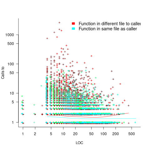
The apparent preponderance of red towards the upper left suggests that frequently called functions are short and contained in files different from the caller. However, the fitted LOESS lines show that the average difference is relatively small. There are many functions of a variety of sizes called once or twice, and few functions called very many times.
The program structure visible in a call graph is cluttered by lots of noise, such as calls to library functions, and the evolution baggage of previous structures. Also, a program may be built from source written in multiple languages (C/C++ is the classic example), and language interface issues can influence organization locally and globally (for instance, in Alibaba’s weex project the function main (in C) essentially just calls serverMain (in C++), which contains lots of code).
I suspect that many call graphs can be mapped to trees (the presence of recursion, though a chain of calls, sometimes comes as a surprise to developers working on a project). Call information needs to be integrated with loops and if-statements to figure out story structures (see section 6.9.1 of my C book). Don’t hold your breath for progress.
I expect that the above patterns are present in other languages. CodeQL supports multiple languages, but CodeQL source targeting one language has to be almost completely reworked to target another language, and it’s not always possible to extract exactly the same information. C/C++ appears have the best support.
Function calls are a component information
Recent Comments