Archive
Formal methods and LLM generated mathematical proofs
Formal methods have been popping up in the news again, or at least on the technical news sites I follow.
Both mathematics and software share the same pattern of usage of formal methods. The input text is mapped to some output text. Various characteristics of the output text are checked using proof assistant(s). Assuming the mapping from input to output is complete and accurate, and the output has the desired characteristics, various claims can then be made about the input text, e.g., internally consistent. For software systems, some of the claims of correctness made about so-called formally verified systems would make soap powder manufacturers blush.
Mathematicians have been using LLMs to help find proofs of unsolved maths problems. Human written proofs are traditionally checked by other humans reading them to verify that the claimed proof is correct. LLMs generated proofs are sometimes written in what is called a formal language, this proof-as-program can then be independently checked by a proof assistant (the Lean proof assistant is a popular choice; Rocq is popular for proofs about software).
Software developers are well aware that LLM generated code contains bugs, and mathematicians have discovered that LLM generated proof-programs contain bugs. A mathematical proof bug involves Lean reporting that the LLM generated proof is true, when the proof applies to a question that is different from the actual question asked. Developers have probably experienced the case where an LLM generates a working program that does not do what was requested.
An iterative verification-and-refinement pipeline was used for LLMs well publicised solving of International Mathematical Olympiad problems.
A cherished belief of fans of formal methods is that mathematical proofs are correct. Experience with LLMs shows that a sequence of steps in a generated proof may be correct, but the steps may go down a path unrelated to the question posed in the input text. Also, proof assistants are programs, and programs invariably contain coding mistakes, which sometimes makes it possible to prove that false is true (one proof assistant currently has 83 bug reports of false being proved true).
It is well known, at least to mathematicians, that many published proofs contain mistakes, but that these can be fixed (not always easily), and the theorem is true. Unfortunately, journals are not always interested in publishing corrections. A sample of 51 reviews of published proofs finds that around a third contain serious errors, not easily corrected.
Human written proofs contain intentional gaps. For instance, it is assumed that readers can connect two steps without more details being given, or the author does not want to deter reviewers with an overly long proof. If LLM generated proofs are checked by proof assistants, then the gap between steps needs to be of a size supported by the assistant, and deterring reviewers is not an issue. Does this mean that LLM generated proof is likely to be human unfriendly?
Software is often expressed in an imperative language, which means it can be executed and the output checked. Theorems in mathematics are often expressed in a declarative form, which makes it difficult to execute a theorem to check its output.
For software systems, my view is that formal methods are essentially a form of  -version programming, with
  . Two programs are written, with one nominated to be called the specification; one or more tools are used to analyse both programs, checking that their behavior is consistent, and sometimes other properties. Mistakes may exist in the specification program or the non-specification program.
Using LLMs to help solve mathematical problems is a rapidly evolving field. We will have to wait and see whether end-to-end LLM generated proofs turn out to be trustworthy, or remain as a very useful aid.
Distribution of small project completion times
Records of project estimates and actual task times show that round numbers are very common. Various possible reasons have been suggested for why actual times are often reported as a round number. This post analyses the impact of round number reports of actual times on the accuracy of estimates.
The plot below shows the number of tasks having a given reported completion time for 1,525 tasks estimated to take 1-hour (code+data):
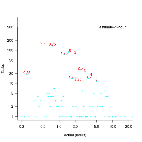
Of those 1,525 tasks estimated to take 1-hour, 44% had a reported completion time of 1-hour, 26% took less than 1-hour and 30% took more than 1-hour. The mean is 1.6 hours and the standard deviation 7.1. The spikiness of the distribution of actual times rules out analytical statistical analysis of the distribution.
If a large task is broken down into, say, smaller tasks, all estimated to take the same amount of time  , what is the distribution of actual times for the large task?
In the case of just two possible actual times to complete each smaller task, some percentage,  , of tasks are completed in actual time
  , and some percentage,
  , completed in actual time
  (with
(with  ). The probability distribution of the large task time,
 ") , for the two actual times case is:
, for the two actual times case is:
=(matrix{2}{1}{N k})(1-p_{t1})^k {p_{t1}}^{N-k}=(matrix{2}{1}{N k}){p_{t2}}^k (1-p_{t2})^{N-k}")
where:  , and
, and  .
.
The right-most equation is the probability distribution of the Binomial distribution, ") . The possible completion times for the large task start at
. The possible completion times for the large task start at  , followed by time increments of .
When there are three possible actual completion times for each smaller task, the calculation is complicated, and become more complicated with each new possible completion time.
A practical approach is to use Monte Carlo simulation. This involves simulating lots of large tasks containing smaller tasks. A sample of tasks is randomly drawn from the known 1,525 task actual times, and these actual times added to give one possible completion time. Running this process, say, 10,000 times produces what is known as the empirical distribution for the large task completion time.
The plot below shows the empirical distribution  smaller 1-hour tasks. The blue/green points show two peaks, the higher peak is a consequence of the use of round numbers, and the lower peak a consequence of the many non-round numbers. If the total times are rounded to 15 minute times, red points, a smoother distribution with a single peak emerges (code+data):

When a large task involves smaller tasks estimated to take a variety of times, the empirical distribution of the actual time for each estimated time can be combined to give an empirical distribution of the large task (see sum_prob_distrib).
Provided enough information on task completion times is available, this technique works does what it says on the tin.
Modelling time to next reported fault
After the arrival of a fault report for a program, what is the expected elapsed time until the next fault report arrives (assuming that the report relates to a coding mistake and is not a request for enhancement or something the user did wrong, and the number of active users remains the same and the program is not changed)? Here, elapsed time is a proxy for amount of program usage.
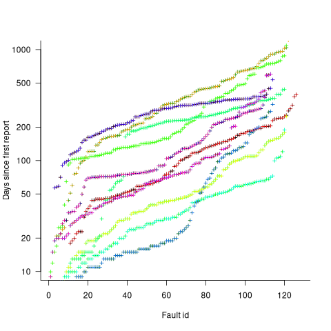
Measurements (here and here) show a consistent pattern in the elapsed time of duplicate reports of individual faults. Plotting the time elapsed between the first report and the n’th report of the same fault in the order they were reported produces an exponential line (there are often changes in the slope of this line). For example, the plot below shows 10 unique faults (different colors), the number of days between the first report and all subsequent reports of the same fault (plus character); note the log scale y-axis (discussed in this post; code+data):
The first person to report a fault may experience the same fault many times. However, they only get to submit one report. Also, some people may experience the fault and not submit a report.
If the first reporter had not submitted a report, then the time of first report would be later. Also, the time of first report could have been earlier, had somebody experienced it earlier and chosen to submit a report.
The subpopulation of users who both experience a fault and report it, decreases over time. An influx of new users is likely to cause a jump in the rate of submission of reports for previously reported faults.
It is possible to use the information on known reported faults to build a probability model for the elapsed time between the last reported known fault and the next reported known fault (time to next reported unknown fault is covered at the end of this post).
The arrival of reports for each distinct fault can be modelled as a Poisson process. The time between events in a Poisson process with rate  has an exponential distribution, with mean
  . The distribution of a sum of multiple Poisson processes is itself a Poisson process whose rate is the sum of the individual rates. The other key point is that this process is memoryless. That is, the elapsed time of any report has no impact on the elapsed time of any other report.
If there are  different faults whose fitted report time exponents are:
  ,
,  …
…  , then summing the Poisson rates,
  , gives the mean
  , for a probability model of the estimated time to next any-known fault report.
To summarise. Given enough duplicate reports for each fault, it’s possible to build a probability model for the time to next known fault.
In practice, people are often most interested in the time to the first report of a previous unreported fault.
tl;dr Modelling time to next previously unreported fault has an analytic solution that depends on variables whose values have to be approximately approximated.
The method used to build a probability model of reports of known fault can be used extended to build a probability model of first reports of currently unknown faults. To build this model, good enough values for the following quantities are needed:
- the number of unknown faults,
 , remaining in the program. I have some ideas about estimating the number of unknown faults, , and will discuss them in another post,
 - the time,
 , needed to have received at least one report for each of the unknown faults. In practice, this is the lifetime of the program, and there is data on software half-life. However, all coding mistakes could trigger a fault report, but not all coding mistakes will have done so during a program’s lifetime. This is a complication that needs some thought,
 - the values of
 ,
,  …
…  for each of the unknown faults. There is some data suggesting that these values are drawn from an exponential distribution, or something close to one. Also, an equation can be fitted to the values of the known faults. The analysis below assumes that the
  for each unknown fault that might be reported is randomly drawn from an exponential distribution whose mean is .
This rate will be affected by program usage (i.e., number of users and the activities they perform), and source code characteristics such as the number of executions paths that are dependent on rarely true conditions.
Putting it all together, the following is the question I asked various LLMs (which uses , rather than ):
There are independent processes. Each process,  , transmits a signal, and the number of signals transmitted in a fixed time interval, , has a Poisson distribution with mean
  for
for  . The values are randomly drawn from the same exponential distribution. What is the cumulative distribution for the time between the successive first signals from the processes.
The cumulative distribution gives the probability that an event has occurred within a given amount of time, in this case the time since the last fault report.
The ChatGPT 5.2 Thinking response (Grok Thinking gives the same formula, but no chain of thought): The probability that the  unknown fault is reported within time
  of the previous report of an unknown fault,
 ") , is given by the following rather involved formula:
, is given by the following rather involved formula:
=1-(a/{a+t})^{N-k}{}_{2}F_1(N-k, k; N+1; t/{a+t})")
where: is the initial number of faults that have not been reported,  , and
, and  is the hypergeometric function.
The important points to note are: the value  decreases as more unknown faults are reported, and the dominant contribution of the value .
Deepseek’s response also makes complicated use of the same variables, and the analysis is very similar before making some simplifications that don’t look right (text of response). Kimi’s response is usually very good, but for this question failed to handle the consequences of .
Almost all published papers on fault prediction ignore the impact of number of users on reported faults, and that report time for each distinct fault has a distinct distribution, i.e., their analysis is not connected to reality.
My 2025 in software engineering
Unrelenting talk of LLMs now infests all the software ecosystems I frequent.
- Almost all the papers published (week) daily on the Software Engineering arXiv have an LLM themed title. Way back when I read these LLM papers, they seemed to be more concerned with doing interesting things with LLMs than doing software engineering research.
- Predictions of the arrival of AGI are shifting further into the future. Which is not difficult given that a few years ago, people were predicting it would arrive within 6-months. Small percentage improvements in benchmark scores are trumpeted by all and sundry.
- Towards the end of the year, articles explaining AI’s bubble economics, OpenAI’s high rate of loosing money, and the convoluted accounting used to fund some data centers, started appearing.
Coding assistants might be great for developer productivity, but for Cursor/Claude/etc to be profitable, a significant cost increase is needed.
Will coding assistant companies run out of money to lose before their customers become so dependent on them, that they have no choice but to pay much higher prices?
With predictions of AGI receding into the future, a new grandiose idea is needed to fill the void. Near the end of the year, we got to hear people who must know it’s nonsense claiming that data centers in space would be happening real soon now.
I attend one or two, occasionally three, evening meetups per week in London. Women used to be uncommon at technical meetups. This year, groups of 2–4 women have become common in meetings of 20+ people (perhaps 30% of attendees); men usually arrive individually. Almost all women I talked to were (ex) students looking for a job; this was also true of the younger (early 20s) men I spoke to. I don’t know if attending meetups been added to the list of things to do to try and find a job.
Tom Plum passed away at the start of the year. Tom was a softly spoken gentleman whose company, PlumHall, sold a C, and then C++, compiler validation suite. Tom lived on Hawaii, and the C/C++ Standard committees were always happy to accept his invitation to host an ISO meeting. The assets of PlumHall have been acquired by Solid Sands.
Perennial was the other major provider of C/C++ validation suites. It’s owner, Barry Headquist, is now enjoying his retirement in Florida.
The evidence-based software engineering Discord channel continues to tick over (invitation), with sporadic interesting exchanges.
What did I learn/discover about software engineering this year?
Software reliability research is a bigger mess than I had previously thought.
I now regularly use LLMs to find mathematical solutions to my experimental models of software engineering processes. Most go nowhere, but a few look like they have potential (here and here and here).
Analysis/data in the following blog posts, from the last 12-months, belongs in my book Evidence-Based Software Engineering, in some form or other (2025 was a bumper year):
Naming convergence in a network of pairwise interactions
Lifetime of coding mistakes in the Linux kernel
Decline in downloads of once popular packages
Distribution of method chains in Java and Python
Modeling the distribution of method sizes
Distribution of integer literals in text/speech and source code
Percentage of methods containing no reported faults
Half-life of Open source research software projects
Positive and negative descriptions of numeric data
Impact of developer uncertainty on estimating probabilities
After 55.5 years the Fortran Specialist Group has a new home
When task time measurements are not reported by developers
Evolution has selected humans to prefer adding new features
One code path dominates method execution
Software_Engineering_Practices = Morals+Theology
Long term growth of programming language use
Deciding whether a conclusion is possible or necessary
CPU power consumption and bit-similarity of input
Procedure nesting a once common idiom
Functions reduce the need to remember lots of variables
Remotivating data analysed for another purpose
Half-life of Microsoft products is 7 years
How has the price of a computer changed over time?
Deep dive looking for good enough reliability models
Apollo guidance computer software development process
Example of an initial analysis of some new NASA data
Extracting information from duplicate fault reports
I visited Foyles bookshop on Charing cross road during the week (if you’re ever in London, browsing books in Foyles is a great way to spend an afternoon).
Computer books once occupied almost half a floor, but is now down to five book cases (opposite is statistics occupying one book case, and the rest of mathematics in another bookcase):

Around the corner, Gender Studies and LGBTQ+ occupies seven bookcases (the same as last year, as I recall):

Programming Punched card machines
Punched card machines, or Tabulating machines, or Unit Record equipment, or according to a 1931 article Super Computing machines, were electromechanical devices that summarised information contained on punched cards (aka tabulating cards). These machines date from 1884, with the publication of Herman Hollerith’s patent application 18840923. In 1948 the electronic valve based IBM 603 calculating punch machine was launched.
The image below (from Wikipedia) shows an IBM 80 column card. When introduced in 1928, the card contained 10 rows, with rows 11 and 12 (known as zone punching positions) added later to support non-digit characters. The paper: “Do Not Fold, Spindle or Mutilate”: A Cultural History of the Punch Card takes a wry look at the social impact of these cards.

Manufacturers sold a range of single purpose Punch machines. Single purposes included: sorting cards, duplicating cards with specified changes to column contents, printing card contents, and simple accounting (adding/subtracting values).
Yes, Punched card machines can be programmed. The vast majority of machines were used by businesses for accounting and stock control, but since the early 1930s a few were used by researchers for scientific computations.
A Punch machine program consisted of cables that directed the flow of electrical signals from one to eighty output sockets (one for each of the 80 columns on a punched card), through various control/manipulation subsystems, to produce an output, e.g., printing a cheque, an itemised invoice, or creating an updated card. The input/output sockets (the terminology of the day was entry/exit sockets) for each subsystem were arranged on the machine’s Control panel (more commonly known as a plugboard).
Each plugboard contains a row of reader output sockets, one for each of the 80 card columns, a row of input sockets that connected to a printing mechanism, and sockets providing input/output for other operations. For example, a connection from, say, the 50’th column of the reader output socket to the 70’th column of the print input socket would print the contents of the 50’th column of the card in the 70’th column of the paper/card output.
The image below (from Wikipedia) shows connections for a program on an IBM 402:

Like many early computers, Punch machine architecture is bit-serial. That is, values are represented as a constant-duration sequence of bits (with the 12 rows of a column forming a card cycle), rather than a parallel sequence of bits (e.g., a byte) all appearing at the same time. The duration of the sequence is driven by the card reader, which moves the card (bottom to top) across a row of metal brushes (one for each column), completing an electric circuit (generating a pulse) when the brush makes contact through a hole in the card.
Once a card cycle completes, the bit sequences are gone (some machines could store a few column values). Some Punch machines read the same card multiple times (three is the maximum I have seen). Multiple readings make it possible to use input from the first/second reading to select the operations to be performed on the input during subsequent readings.
An example of the need for multiple reads. Holes in the zone punching positions may specify an alphabetic character or a special data specific meaning, e.g., accounting records could indicate that a column value is a credit rather than a debit by punching a hole in the 11’th row of the appropriate column. To maintain backwards compatibility, the zone punching positions appear near the top of the punch card, and are read last, leaving the digits pulses unchanged. If a zone punching position has a special meaning, the first read is used to detect whether, say, the 11’th row contains a hole, and the digit value is obtained on the second read (see X Elimination on page 126).
Punch machine programs did not support loops. Loops are implemented by including a human in the chain of execution. The body of the loop performs a calculation on the input cards, writing the results to new cards. These new cards are moved to the input hopper, and the program run again, iterating until the desired accuracy is obtained (or not).
Naming convergence in a network of pairwise interactions
While naming and categorizing things are perhaps the two most contentious issues in software engineering, there is often a great deal of similarity in the names and categorizes used by unconnected groups. These characteristics of naming and categorization are general observed behaviors across cultures and languages, with software engineering being a particular example.
Studies have found that a particular name for a thing is likely to become adopted by a group, if around 25% of its members actively promote the use of the name. The terms tipping point and critical mass have been applied to the 25% quantity.
What factors could cause 25% of the members of a group to select a particular name, and why does a tipping point occur at around this percentage?
The paper Experimental evidence for scale-induced category convergence across populations by Douglas Guilbeault (PhD thesis behind the paper), Andrea Baronchelli, and Damon Centola experimentally investigated factors that can cause a name to be adopted by 25% of a group’s members, and the researchers proposed a model that exhibits behavior similar to the experimental results (the supplement contains the technical details).
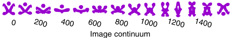
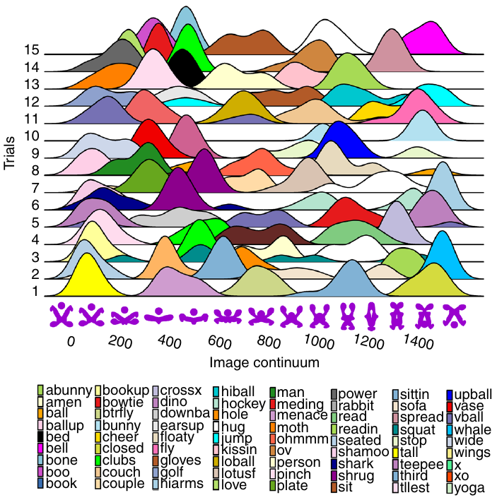
The experiment asked subjects to play the “Grouping Game”. The 1,480 online subjects were divided into networks containing either 2, 6, 8, 24 or 50 members. The interaction between members of a network only occurred via randomly selected pairs (the same pair for the network of two), with one person designated as the speaker and the other as the hearer. A pair saw three randomly selected images, such as the one below. For the speaker only, one of the images was highlighted, and they had to give a name containing at most six characters to the image. The hearer saw the name given by the speaker to one of the images, and had 30 seconds to choose the image they considered to have been named. If the image selected by the hearer was the one named by the speaker, both received a small payment, otherwise an even smaller amount was deducted from their final payment. Each subject played 100 rounds with the randomly chosen members of their network.

The images were created as a series of 50+ distinct patterns whose shape slowly morphed along a continuum, as in the following image:
The experimental results were that larger networks converged to a consistent, within group, naming of the images (using a few names), while smaller groups rarely converged and used many different names. The researchers proposed that as the network size grew, common names were encountered more often than rarer names, increasing the likelihood of reaching a tipping point. This behavior is similar to the birthday paradox, where there is a 50% probability that in a room of 23 people, two people will share the same birthday.
In the experiment, some networks included confederates trained to use a small subset of names, i.e., the researchers created a common set of names. It was hypothesized built-in human preferences would produce common patterns in the real world that, for larger groups, would cause tipping points to occur, amplifying the more common patterns to become group norms.
The supplement to the paper develops a theoretical model based on the probability of identical items being contained in a sample of  items, when sampling without replacement. The solution involves the hypergeometric distribution, which is difficult to deal with analytically, so simulation is needed. The results show a tipping point at around 25%.
The plot below shows a density plot for one 50-subject network over 15 trials (after 100 rounds of pairwise interaction), with each color denoting one of the 14 chosen names (height of the curve denotes likelihood of the same name being chosen for that image; code and data):
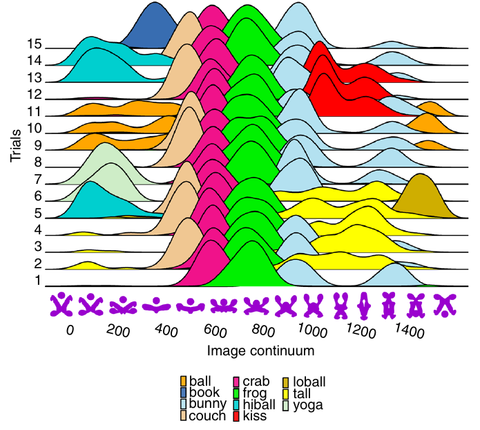
This plot shows that the same name is often used across trials, and naming boundaries between some images.
The plot below shows a density plot for one 2-subject network over 15 trials (after 100 rounds of pairwise interaction), with each color denoting one of the 72 chosen names (height of the curve denotes likelihood of the same name being chosen for that image; code and data):
Here there is no consistent naming across trials, a much greater diversity of names appearing, and no obvious naming boundaries between images.
Christmas books for 2025
My rate of book reading has remained steady this year, however, my ability to buy really interesting books has declined. Consequently, the list of honourable mentions is longer than the main list. Hopefully my luck/skill will improve next year. As is usually the case, most book were not published in this year.
Liberal Fascism: The secret history of the Left from Mussolini to the Politics of Meaning by Jonah Goldberg is reviewed in a separate post.
Oxygen: The molecule that made the world by Nick Lane, a professor of evolutionary biochemistry, published in 2016. The book discusses changes in the percentage of oxygen in the Earth’s atmosphere over billions of years and the factors that are thought to have driven these changes. The content is at the technical end of popular science writing. The author is a strong proponent that life (which over a billion or so years produced most of the oxygen in the atmosphere) originated in hydrothermal vents, not via lightening storms in the Earth’s primordial atmosphere (as suggested by the Miller–Urey experiment). The Wikipedia article on the origins of life contains a lot more words on the Miller–Urey experiment.
“By the Numbers: Numeracy, Religion and the Quantitative Transformation of Early Modern England” by Jessica Marie Otis, a professor of history, published in 2024. Here, early modern England starts around 1543 with the publication of an arithmetic textbook, The Ground of Artes, that was republished 45 times up until 1700. As the title suggests, the book discusses the factors driving the spread of numeracy into the general population, e.g., the need for traders and organizations to keep accounts, and the people to keep track of time. For the general reader, the book is rather short at 160 readable pages. Historians get to enjoy the 51 pages of notes and 37 pages of bibliography.
For insightful long, discursive book reviews that are often more interesting than the books themselves (based on those I have purchased), see: Mr. and Mrs. Psmith’s Bookshelf. This year, Astral Codex ran a Non-Book Review Contest.
The blog Worshipping the Future by Helen Dale and Lorenzo Warby continues to be an excellent read. It is “… a series of essays dissecting the social mechanisms that have led to the strange and disorienting times in which we live.” The series is a well written analysis that attempts to “… understand mechanisms of how and the why, …” of Woke.
As an aside, one of the few pop cds I bought this year turned out to be excellent: “PARANOÏA, ANGELS, TRUE LOVE” by Christine and the Queens.
Honourable mentions
The Knowledge: How to Rebuild Our World from Scratch by Lewis Dartnell, an astrobiologist. Assuming you are among the approximately 5% of people still alive after civilizations collapses (the book does not talk about this, but without industrial scale production of food, most people will starve to death), how can useful modern day items (i.e., available in the last hundred years or so) be created? Items include ammonia-based fertilizer, electricity, radio receiver and simple drugs. The processes sound a lot easier to do than they are likely to be in practice (manufacturing processes invariably make use of a lot of tacit knowledge), but then it is a popular book covering a lot of ground. It’s really a list of items to consider, along with some starting ideas.
“Goodbye, Eastern Europe: An Intimate History of a Divided Land” by Jacob Mikanowski, a historian and science writer, published in 2023. A history of Eastern Europe from the first century to today, covering the countries encircled by Germany, the Baltic Sea, Russia, and the Black Sea/Mediterranean. The story is essentially one of migrations, and mass slaughters, with the accompanying creation and destruction of cultures. Harrowing in places. It’s no wonder that the people from that part of the world cling to whatever roots they have.
“Reframe Your Brain: The User Interface for Happiness and Success” by Scott Adams of Dilbert fame, published in 2023. To quote Wikipedia: “Cognitive reframing is a psychological technique that consists of identifying and then changing the way situations, experiences, events, ideas and emotions are viewed.” This book contains around 200 reframes of every day situations/events/emotions, with accompanying discussion. Some struck me as a bit outlandish, but sometimes outlandish has the desired effect.
Details on your best books of the year very welcome in the comments.
Lifetime of coding mistakes in the Linux kernel
What is the lifetime of coding mistakes in the Linux kernel? Some coding mistakes result in fault reports (some of which are fixed), while many are removed when the source that contains them is deleted/changed during ongoing development.
After fixing the coding mistake(s) in the kernel that generated a reported fault, developer(s) log the commit that introduced the coding mistake, along with the commit that fixed it. This logging started in 2013, and I only found out about it this week. To be exact, I discovered the repo: A dataset of Linux Kernel commits created by Maes Bermejo, Gonzalez-Barahona, Gallego, and Robles.
The log contains the commit hashes for the 90,760 fixes made to the 63 mainline kernel versions from 3.12 to 6.13. The complete log of 1,233,421 commits has to be searched to extract the details, e.g., date, lines added, etc.
The kernel development process involves regular release cycles of around 80 days. Developers submit the code they want to be included in the next release, this goes through a series of reviews, with Linus making the final decision.
The following analysis is based on the coding mistakes introduced between successive kernel releases, e.g., version 3.13 coding mistakes are those introduced into the source between 4 Nov 2013 (the day after version 3.12 was released) and 19 Jan 2014 (when version 3.13 was released). Code will have been worked on, and mistakes created/fixed, before it reached the kernel, which ensures some level of maturity.
The number of people working with pre-release code is likely to be tiny, compared to the number running released kernels. Consequently, the characteristics of coding mistake lifetime is expected to be different pre/post release, if only because more users are likely to report more faults.
The plot below shows the pre-release daily mistake fixed density against days since start of work on the current release, the red line is a fitted regression line mapped to density (fitted regression is a biexponential; code and data):
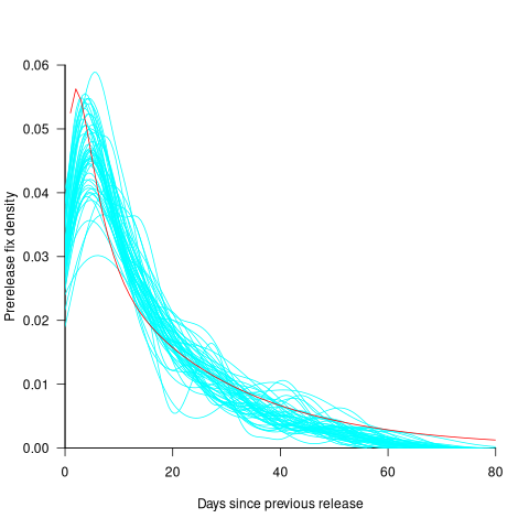
For all versions, the prior to release daily fix rate follows a consistent pattern: Most fixes occur in the first few days, with roughly an exponential decline to the release date.
The following analysis builds a broad brush model of cumulative fixes over time across 53 mainline kernel releases (the final 10 releases were not included because of their relatively short history).
The number of users of a new kernel takes time to increase as it percolates onto systems, e.g., adopted by Linux distributions and then installed by users, or installed by cloud providers. Eventually, code first included in a particular version will be running on most systems.
The post release daily fix rate is best modelled using the cumulative number of fixes, i.e., total number of fixes up to a given day since release. The models fitted below are based on dividing the post release cumulative fixes into before/after 200 days since release. The 200-day division is a round number (technically, a nearby value may provide a better fit) that supports the fitting of good quality before/after regression models. Averaged over all releases, 42% of fixes occurred within 200-days, and 58% after 200-days.
The plot below shows the cumulative number of post-release fixed faults, in red, for various kernel versions, with fitted regression lines in green and blue (grey line is at 200-days; code and data):

The equation fitted to the before 200-days fixes had the following form:
}")
where:  is a kernel version specific constant; see plot below.
The equation fitted to the after 200-days fixes had the following form:

where:  is a kernel version specific constant; see plot below.
Approximately, after release, the cumulative fix rate starts out quadratic in elapsed days, with the rate decreasing over time, until after 200-days the rate settles down to following the cube-root of days.
Comparing the number of post-release fixes across versions, there is a lot more variability in the first 200-days (i.e., the model fit to the data is sometimes very poor), relatively to after 200-days (where the model fit is consistently good).
Each kernel release has its own characteristics, parameterised by the values , and in the above equations. The plot below shows these values across versions, with red for , blue/green for , and grey line showing normalised LOC added/changed in the release (code and data):
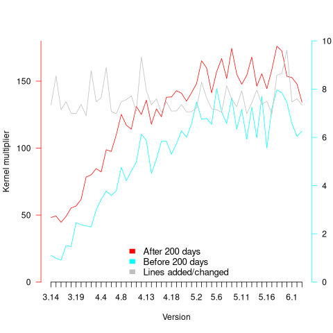
The plot clearly shows a large increase in the number of fixes between kernel version 3.14 and later versions. The before 200-days rate (blue/green) increase by a factor of seven, while the after 200-days rate increased by a factor of three.
Is this increase driven by some underlying factor in kernel development, or is it an external factor such as an increase in the number of users (more users leads to more faults reports), or the extensive post-release fuzz testing that is now common.
The number of lines of code added/changed, indicated by the grey line (shifted to fit plot axes) cannot be added to the fitted models because they exactly correlate with their respective version.
What is driving the long-term rate of fixes, i.e., cube-root of elapsed days?
Actually, what people are really want to know is what can be done to reduce the number of fixes required after release. When people ask me this, my usual reply is: “Spend more on testing”.
The probability of a coding mistake causing a fault report is decreasing: fixes reduce the number of remaining mistakes, and source added in one kernel version may be removed in a later version.
Perhaps the set of input behaviors is growing, producing the distinct conditions needed to trigger different coding mistakes, or the faults are occurring but are only reported when experienced by a small subset of users.
As always, more data is needed.
Update
Some data on Linux kernel use by AWS.
Decline in downloads of once popular packages
What happens to the popularity of Open source packages, measured in monthly downloads, once they cease to be updated or attract new users?
If the software does not have any competition within its domain, there is no reason why its popularity should decline. In practice, there are usually alternative packages offering the same or similar functionality. Even when alternatives are available, existing practice and sunk costs can slow migration. A year or so after I started using Asciidoc to write by Software Engineering book, the author announced that he was no longer going to update the software; initially there was no alternative, but the software did what I wanted, and I have been happily using it over the last 12 years.
The paper: Do All Software Projects Die When Not Maintained? Analyzing Developer Maintenance to Predict OSS Usage by Emily Nguyen measured the monthly downloads, commits and other characteristics of 38K GitHub packages having at least 10K downloads during any month between January 2015 and December 2020. The data made available (more here) is a subset, i.e., downloads for 1,583 projects starting in May 2015.
The author investigated the connection between various project characteristics (focusing on commits or lack thereof in particular) and downloads by fitting a Cox proportional hazards model.
The plot below shows the 67 monthly downloads for a selection of packages; the red line is a fitted local regression used to smooth the data (code and data):

Reasons for a decline from a peak number of downloads include: competition from alternative packages, change of fashion, and market saturation, or perhaps the peak was caused by a one-off event. Whatever the reason for a peak+decline, my interest is learning about patterns in the rate of decline.
Some of the monthly package downloads in the above plot have an obvious peak and decline, with others continually increasing, and others having multiple peaks. The following algorithm was used to select packages having a peak followed by a decline, based on the predicted values from a fitted loess model:
- find the month with the most downloads, this is the primary peak,
- if this month is within 10 months of the end of the measurement period, this is not a peak/decline package,
- does a secondary peak exist? A secondary peak is a month containing the most downloads from 10 months after the end of the primary peak, where the number of downloads is within 66% of the primary peak downloads,
- the secondary peak becomes the primary peak, provided it is not within 10 months of the end of the measurement period.
The final fraction of the primary peak is the average monthly download during the last three months divided by the peak month downloads.
The plot below shows the 693 packages whose final fraction of peak was below 0.6 against months from peak to the last month (at the end of 2020), with the red line showing a fitted regression of the form  (code and data):

As the above plot shows, there don’t appear to be any patterns in the decline of package downloads, and  is a poor predictor of fraction of peak.
Perhaps a more sophisticated peak+decline selection algorithm will uncover some patterns. Both ChatGPT (its generated python script failed) and Grok (very wrong answers) failed miserably at classifying the plots. Deepseek will only process images to extract text.
Occurrence of binary operator overloading in C++
Operator overloading, like many programming language constructs, was first supported in the 1960s (Algol 68 also provided a means to specify a precedence for the operator). C++ is perhaps the most widely used language supporting operator overloading; but not redefining their precedence.
I have always thought that operator overloading was more talked about than actually used (despite its long history, I have not been able to find any published usage information). A previous post noted that the CodeQL databases hosted by GitHub provides the data needed to measure usage, and having wrestled with the documentation (ql scripts used), C++ operator overload usage data is available.
The table below shows the total uses of overloaded and ‘usual’ binary operators in the source code (excluding headers) of 77 C++ repositories on GitHub (the 100 repositories C/C+ MRVA). The table is ordered by total occurrences of overloads, with the Percentage column showing the percentage use of overloaded operators against the total for the respective operator (i.e.,  ; code and data):
Binary Overload Usual Total Percentage << 103,855 20,463 124,318 83.5 == 21,845 118,037 139,882 15.6 != 14,749 69,273 84,022 17.6 * 12,849 57,906 70,755 18.2 + 10,928 103,072 114,000 9.6 && 8,183 64,148 72,331 11.3 - 5,064 77,775 82,839 6.1 <= 3,960 18,344 22,304 17.8 & 3,320 27,388 30,708 10.8 < 1,351 93,393 94,744 1.4 >> 1,082 11,038 12,120 8.9 / 1,062 29,023 30,085 3.5 > 537 44,556 45,093 1.2 >= 473 27,738 28,211 1.7 | 293 13,959 14,252 2.0 ^ 71 1,248 1,319 5.4 <=> 13 12 25 52.0 % 11 9,338 9,349 0.1 || 9 53,829 53,838 0.017 |
Use of the overloaded << operator is driven by standard library I/O, rather than left shifting.
There are seven operators where 10-20% of the usage is overloaded, which is a lot higher than I was expecting (not that I am a C++ expert).
How much does overloaded binary operator usage vary across projects? In the plot below, each vertical colored violin plot shows the distribution of overload usage for one operator across all 77 projects (the central black lines denote the range of the central 50% of the points; code and data):

While there is some variation between these 77 projects, in most cases a non-trivial percentage of an operator's usage is overloaded.
Recent Comments