Uncertainty in data causes inconsistent models to be fitted
Does software development benefit from economies of scale, or are there diseconomies of scale?
This question is often expressed using the equation:  . If
. If  is less than one there are economies of scale, greater than one there are diseconomies of scale. Why choose this formula? Plotting project effort against project size, using logs scales, produces a series of points that can be sort-of reasonably fitted by a straight line; such a line has the form specified by this equation.
Over the last 40 years, fitting a collection of points to the above equation has become something of a rite of passage for new researchers in software cost estimation; values for have ranged from 0.6 to 1.5 (not a good sign that things are going to stabilize on an agreed value).
This article is about the analysis of this kind of data, in particular a characteristic of the fitted regression models that has been baffling many researchers; why is it that the model fitted using the equation is not consistent with the model fitted using  , using the same data. Basic algebra requires that the equality
  be true, but in practice there can be large differences.
The data used is Data set B from the paper Software Effort Estimation by Analogy and Regression Toward the Mean (I cannot find a pdf online at the moment; Code+data). Another dataset is COCOMO 81, which I analysed earlier this year (it had this and other problems).
The difference between and  is a result of what most regression modeling algorithms are trying to do; they are trying to minimise an error metric that involves just one variable, the response variable.
In the plot below left a straight line regression has been fitted to some Effort/Size data, with all of the error assumed to exist in the  values (dotted red lines show the residual for each data point). The plot on the right is another straight line fit, but this time the error is assumed to be in the
  values (dotted green lines show the residual for each data point, with red line from the left plot drawn for reference). Effort is measured in hours and Size in function points, both scales show the
  of the actual value.
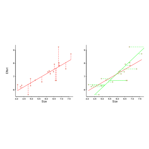
Regression works by assuming that there is NO uncertainty/error in the explanatory variable(s), it is ALL assumed to exist in the response variable. Depending on which variable fills which role, slightly different lines are fitted (or in this case noticeably different lines).
Does this technical stuff really make a difference? If the measurement points are close to the fitted line (like this case), the difference is small enough to ignore. But when measurements are more scattered, the difference may be too large to ignore. In the above case, one fitted model says there are economies of scale (i.e.,  ) and the other model says the opposite (i.e.,
  , diseconomies of scale).
There are several ways of resolving this inconsistency:
- conclude that the data contains too much noise to sensibly fit a a straight line model (I think that after removing a couple of influential observations, a quadratic equation might do a reasonable job; I know this goes against 40 years of existing practice of do what everybody else does…),
- obtain information about other important project characteristics and fit a more sophisticated model (characteristics of one kind or another are causing the variation seen in the measurements). At the moment information is being used to explain all of the variance in the data, which cannot be done in a consistent way,
- fit a model that supports uncertainty/error in all variables. For these measurements there is uncertainty/error in both and ; writing the same software using the same group of people is likely to have produced slightly different Effort/Size values.
There are regression modeling techniques that assume there is uncertainty/error in all variables. These are straight forward to use when all variables are measured using the same units (e.g., miles, kilogram, etc), but otherwise require the user to figure out and specify to the model building process how much uncertainty/error to attribute to each variable.
In my Empirical Software Engineering book I recommend using simex. This package has the advantage that regression models can be built using existing techniques and then ‘retrofitted’ with a given amount of standard deviation in specific explanatory variables. In the code+data for this problem I assumed 10% measurement uncertainty, a number picked out of thin air to sound plausible (its impact is to fit a line midway between the two extremes seen in the right plot above).
https://www.simula.no/sites/simula.no/files/publications/SE.4.Joergensen.2003.a.pdf
That link takes you to a PDF of ” Software Effort Estimation by Analogy and Regression Toward the Mean”. The site has PDFs of many fascinating papers, including the result that effort predictions in work-HOURS are different from effort predictions in work-DAYS.
@Richard A. O’Keefe
Thanks for the link. Joergensen has done some very good work and is currently the most quote author in my data collection.