Distribution of uptimes for high-performance computing systems
Computers break down every now and again and this is a serious problem when an application needs runs on thousands of individual computers (nodes) plugged together; lots more hardware creates lots more opportunity for a failure that renders any subsequent calculations by working nodes possible wrong. The solution is checkpointing; saving the state of each node every now and again, and rolling back to that point when a failure occurs. Picking the optimal interval between checkpoints requires knowledge the distribution of node uptimes, what is it?
Short answer: Node uptimes have a negative binomial distribution, or at least five systems at the Los Alamos National Laboratory do.
The longer answer is below as another draft section from my book Empirical software engineering with R. As always comments and pointers to more data welcome. R code and data here.
Distribution of uptimes for high-performance computing systems
Today’s high-performance computing systems are created by connecting together lots of cpus. There is a hierarchy to the connection in that many cpus may populate a single board, several boards may be fitted into a rack unit, several rack units into a cabinet, lots of cabinets lined up in a row within a room and more than one room in a facility. A common operating unit is the node, effectively a computer on which an operating system is running (the actual hardware involved may be a single or multi processor cpu). A high-performance system is built from thousands of nodes and an application program may run on compute nodes from more than one facility.
With so many components, failures occur on a regular basis and long running applications need to recover from such failures if they are to stand a reasonable chance of ever completing.
Applications running on the systems installed at the Los Alamos National Laboratory create checkpoints at regular intervals, writing data needed to do a full restore to storage. When a failure occurs an application is restarted from its most recent checkpoint, one node failure causes all nodes to be rolled back to their most recent checkpoint (all nodes create their checkpoints at the same time).
A tradeoff has to be made between frequently creating checkpoints, which takes resources away from completing execution of the application but reduces the amount of lost calculation, and infrequent checkpoints, which diverts less resources but incurs greater losses when a fault occurs. Calculating the optimum checkpoint interval requires knowing the distribution of node uptimes and the following analysis attempts to find this distribution.
Data
The data comes from 23 different systems installed at the Los Alamos National Laboratory (LANL) between 1996 and 2005. The total failure count for most of the systems is of the order of a few hundred; there are five systems (systems 2, 16, 18, 19 and 20) that each have several thousand failures and these are the ones analysed here.
The data consists of failure records for every node in a system. A failure record includes information such as system id, node number, failure time, restored to service time, various hardware characteristics and possible root causes for the failure. Schroeder and Gibson <book Schroeder_06> performed the first analysis of the dataset and provide more background details.
Is the data believable?
Failure records are created by operations staff when they are notified by the automated monitoring system that a failure has been detected. Given that several people are involved in the process <book LANL_data_06> it seems unlikely that failures will go unreported.
Some of the failure reports have start times before the given node was returned into service from the previous failure; across the five systems this varied between 0.4% and 2.5%. It is possible that these overlapping failures are caused by an incorrectly attempt to fix the first failure, or perhaps they are data entry errors. This error rate is comparable with human error rates for low stress/non-critical work
The failure reports do not include any information about the application software running on the node when it failed; the majority of the programs executed are large-scale scientific simulations, such as simulations of nuclear stockpile stability. Thus it is not possible to accurately calculate the node MTBF for an executing application. LANL say <book LANL_data_06> that the applications “… perform long periods (often months) of CPU computation, interrupted every few hours by a few minutes of I/O for check-pointing.”
Predictions made in advance
The purpose of this analysis is to find the distribution that best fits the node uptime data, i.e., the time interval between failures of the same node.
Your author is not aware of any empirically based theory that predicts the uptime of high performance computing systems. The Poisson and exponential distributions are both frequently encountered in the analysis of hardware failures and it is always comforting to fit in with existing expectations.
Applicable techniques
A [Cullen and Frey test] matches a dataset’s skew and kurtosis against known distributions (in the case of the descdist function in the fitdistrplus package this is a handful of commonly encountered distributions); the fitdist function in the same package can be used to fit the data to a specified distribution.
Results
The table below lists some basic properties of each of the systems analysed. The large difference in mean/median uptimes between some systems is caused by very fat tails in the uptime distribution of some systems, see [LANL-node-uptime-binned].
| System | Nodes | Failures | Mean | Median |
|---|---|---|---|---|
|
2
|
49
|
6997
|
133
|
377
|
|
16
|
16
|
2595
|
89
|
229
|
|
18
|
823
|
3014
|
2336
|
4147
|
|
19
|
738
|
2344
|
2376
|
4069
|
|
20
|
323
|
2063
|
653
|
2544
|
If there are any significant changes in failure rate over time or across different nodes in a given system it could have a significant impact on the distribution of uptime intervals. So we first check to large differences in failure rates.
Do systems experience any significant changes in failure rate over time?
The plot below shows the total number of failures, binned using 30-day periods, for the five systems. Two patterns that stand out are system 20 which experienced many failures during the first few months and then settled down, and system 2’s sudden spike in failures around month 23 before settling down again. This analysis is intended to be broad brush and does not get involved with details of specific systems, but these changes in failure frequency suggest that the exact form of any fitted distribution may change over time in turn potentially leading to a change of checkpoint interval.
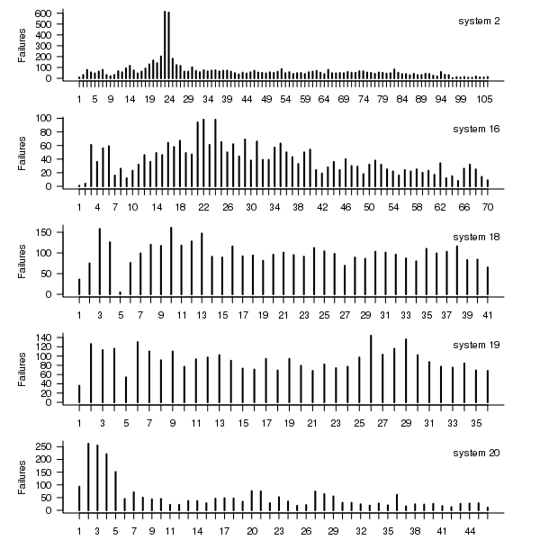
Figure 1. Total number of failures per 30-day interval for each LANL system.
Do some nodes failure more often than others?
The plot below shows the total number of failures for each node in the given system. Node 0 has many more failures than the other nodes (for node 0 of system 2 most of the failure data appears to be missing, so node 1 has the most failures). The distribution suggested by the analysis below is not changed if Node 0 is removed from the dataset.
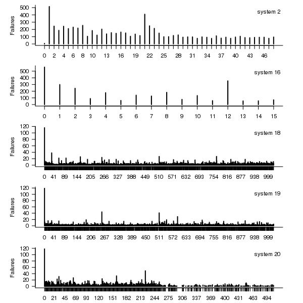
Figure 2. Total number of failures for each node in the given LANL system.
Fitting node uptimes
When plotted in units of 1 hour there is a lot of variability and so uptimes are binned into 10 hour units to help smooth the data. The number of uptimes in each 10-hour bin forms a discrete distribution and a [Cullen and Frey test] suggests that the negative binomial distribution might provide the best fit to the data; the Scroeder and Gibson analysis did not try the negative binomial distribution and of those they tried found the Weilbull distribution gave the best fit; the R functions were not able to fit this distribution to the data.
The plot below shows the 10-hour binned data fitted to a negative binomial distribution for systems 2 and 18. Visually the negative binomial distribution provides the better fit and the Akaiki Information Criterion values confirm this (see code for details and for the results on the other systems, which follow one of the two patterns seen in this plot).
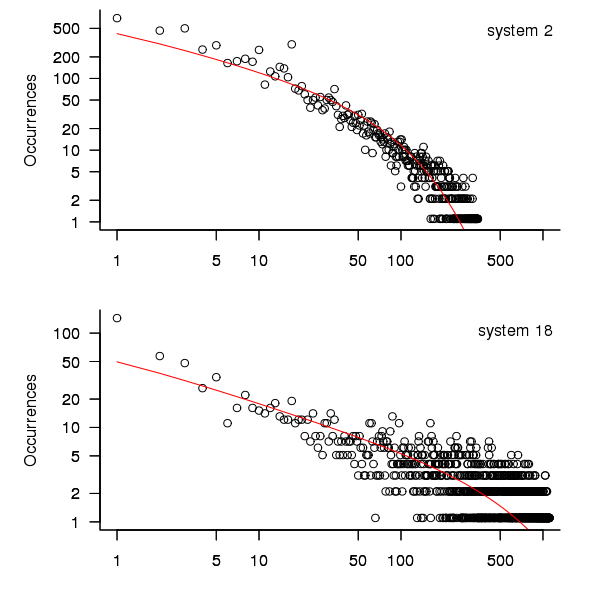
Figure 3. For systems 2 and 18, number of uptime intervals, binned into 10 hour interval, red line is fitted negative binomial distribution.
The negative binomial distribution is also the best fit for the uptime of the systems 16, 19 and 20.
The Poisson distribution often crops up in failure analysis. The quality of fit of a Poisson distribution to this dataset was an order of worse for all systems (as measured by AIC) than the negative binomial distribution.
Discussion
This analysis only compares how well commonly encountered distributions fit the data. The variability present in the datasets for all systems means that the quality of all fitted distributions will be poor and there is no theoretical justification for testing other, non-common, distributions. Given that the analysis is looking for the best fit from a chosen set of distributions no attempt was made to tune the fit (e.g., by forming a zero-truncated distribution).
Of the distributions fitted the negative binomial distribution has the lowest AIC and best fit visually.
As discussed in the section on [properties of distributions] the negative binomial distribution can be generated by a mixture of [Poisson distribution]s whose means have a [Gamma distribution]. Perhaps the many components in a node that can fail have a Poisson distribution and combined together the result is the negative binomial distribution seen in the uptime intervals.
The Weilbull distribution is often encountered with datasets involving some form of time between events but was not seen to be a good fit (for a continuous distribution) by a Cullen and Frey test and could not be fitted by the R functions used.
The characteristics of node uptime for two systems (i.e., 2 and 16) follows what might be thought of as a typical distribution of measurements, with some fattening in the tail, while two systems (i.e., 18 and 19) have very fat tails with indeed and system 20 sits between these two patterns. One system characteristic that matches this pattern is the number of nodes contained within it (with systems 2 and 16 having under 50, 18 and 19 having over 1,000 and 20 having around 500). The significantly difference in the size of the tails is reflected in the mean uptimes for the systems, given in the table above.
Summary of findings
The negative binomial distribution, of the commonly encountered distributions, gives the best fit to node uptime intervals for all systems.
There is over an order of magnitude variation in the mean uptime across some systems.
Recent Comments