Archive
Why is Cobol still popular in Japan?
Rummaging around the web for empirical software engineering data, I found a survey of programming language usage in Japan. This survey (based on 505 projects in 24 companies) has Cobol in the number two slot for 2012, a bit higher than I would have expected (it very rarely appears at all in US/UK ‘popularity’ lists):
Language       Projects
Java             822  28.2%
COBOL            464  15.9%
VB               371  12.7%
C                326  11.2%
Other languages  208   7.1%
C++              189   6.5%
Visual Basic.NET 136   4.7%
Visual C++       105   3.6%
C#               101   3.5%
PL/SQL            57   2.0%
Pro*C             23   0.8%
Excel(VBA)        18   0.6%
Developer2000     17   0.6%
ABAP              15   0.5%
HTML              14   0.5%
Delphi            11   0.4%
PL/I              10   0.3%
Perl              10   0.3%
PowerBuilder       7   0.2%
Shell              7   0.2%
XML                6   0.2%
A quick overview of Cobol for those readers who have never encountered it.
Cobol is a domain specific language ideally suited for business data processing in the 1960/70/80/90s. During this period computer memory was often measured in kilobytes, data came in an unbelievably wide range of different formats, operations on data mostly involved sorting and basic arithmetic, and output data format was/is very important. By “unbelievably wide range” think of lots of point-of-sale vendors deciding how their devices would write data to punch cards/paper tape/magnetic tape, just handling the different encodings that have been used for the plus/minus sign can make the head spin; combine the requirement that programs handle different data formats with tiny computer memory capacity, and you get data structure overlays that make C programmers look like rank amateurs, all the real action in Cobol programs occurs in the DATA DIVISION.
So where are we today? Companies use computers to solve a wider range of problems don’t they (so even if Cobol usage stayed the same its percentage usage should be low)? If point-of-sale terminals still produce a wide range of weird and wonderful data formats, isn’t it easy enough to write the appropriate libraries to convert (and we have much more storage these days)?
Why might Cobol still be so popular in Japan (and perhaps elsewhere, if anybody over 25 was included in the survey)? Some ideas:
- Cobol is still the best language to use for business data processing,
- the sample is not representative of the Japanese software development industry. As a government body perhaps the Information-Technology Promotion Agency primarily deals with large well established companies; the data came from a relatively small number of companies (i.e., 24),
- the Japanese are known for being conservative and maintaining traditions. Change is almost considered a necessity here in the West, this has led to the use of way too many programming languages in industry (I have previously written about what a mistake it is to invent a new language).
Sampling is now an issue in software engineering research
Data analysis in software engineering often has to make do with measurements extracted from the handful of measurable/measured instances at hand, but every now and again the abundance of stuff to measure is such that a subset has to be selected. How should the subset be selected?
Population sampling is a well established part of statistics, and a variety of terms have sprung up to label the various strategies used. I think ‘Accidental sampling’ accurately describes the provenance of many software engineering datasets seen in research papers and some of my work. It is quite common to see academic papers using exactly the same sample as previously published papers, perhaps a new term is needed to describe using samples that are identical to those used in previously papers: lazy sampling, coat-tail sampling…
Program source code, which was once so hard to obtain in any significant quantity, is now available by the terabyte load, a population that all but the fastest analysis and most general of questions warrant processing as a whole.
The question being asked can itself intrinsically lead to a reduction in the size of the population, e.g., properties of programs written in X, or programs with more than 10 active developers.
What should be the unit of sampling? The package making up a standalone system/library is a common choice (e.g., all the files in the tar or zip archive from which binaries are built); this can result in unexpected source files being included in the measurement process, such as test programs. A less common choice is to use individual source files as the sampling unit (it is so much easier to randomly select a list of packages, download, extract and measure them one by one).
Are the source file characteristics of the contents of 1,000 packages statistically very similar to 25,000 files obtained by randomly selecting 1 file from 25,000 packages? I don’t know.
A recent paper by Nagappan, Zimmermann and Bird proposes a sampling algorithm which looks like quota or coverage sampling in that candidate similarity to the current sample is used to decide whether to add that candidate (too much similarity results in exclusion). The authors misleadingly associate the term ‘representativeness’ with this algorithm, where common statistical usage of representative requires that if 40% of a population have attribute Z then 40% of a sample’s members will have this attribute (within sampling tolerances).
If software engineering research is to be useful to commercial software engineering, any discoveries need to be applicable to samples outside of those used in the original analysis. At the moment researchers are having a hard enough time finding any useful patterns in their data, this is not a reason to continue with the practice of coat-tail sampling and we all need to start addressing sampling issues.
Break even ratios for development investment decisions
Developers are constantly being told that it is worth making the effort when writing code to make it maintainable (whatever that might be). Looking at this effort as an investment what kind of return has to be achieved to make it worthwhile?
Short answer: The percentage saving during maintenance has to be twice as great as the percentage investment during development to break even, higher ratio to do better.
The longer answer is below as another draft section from my book Empirical software engineering with R book. As always comments and pointers to more data welcome. R code and data here.
Break even ratios for development investment decisions
Upfront investments are often made during software development with the aim of achieving benefits later (e.g., reduced cost or time). Examples of such investments include spending time planning, designing or commenting the code. The following analysis calculates the benefit that must be achieved by an investment for that investment to break even.
While the analysis uses years as the unit of time it is not unit specific and with suitable scaling months, weeks, hours, etc can be used. Also the unit of development is taken to be a complete software system, but could equally well be a subsystem or even a function written by one person.
Let  be the original development cost and
  the yearly maintenance costs, we start by keeping things simple and assume is the same for every year of maintenance; the total cost of the system over
  years is:

If we make an investment of  % in reducing future maintenance costs with the expectations of achieving a benefit of
  %, the total cost becomes:
 + y*m*(1+i)*(1-b)")
and for the investment to break even the following inequality must hold:
 + y*m*(1+i)*(1-b) < d + y*m")
expanding and simplifying we get:

or:

If the inequality is true the ratio  is the primary contributor to the right-hand-side and must be greater than 1.
A significant problem with the above analysis is that it does not take into account a major cost factor; many systems are replaced after a surprisingly short period of time. What relationship does the ratio need to have when system survival rate is taken into account?
Let  be the percentage of systems that survive each year, total system cost is now:

where *(1-b)")
Summing the power series for the maximum of years that any system in a company’s software portfolio survives gives:
}/{1 - s}")
and the break even inequality becomes:
} < {b}/{i} + b")
The development/maintenance ratio is now based on the yearly cost multiplied by a factor that depends on the system survival rate, not the total maintenance cost
If we take >= 5 and a survival rate of less than 60% the inequality simplifies to very close to:

telling us that if the yearly maintenance cost is equal to the development cost (a situation more akin to continuous development than maintenance and seen in 5% of systems in the IBM dataset below) then savings need to be at least twice as great as the investment for that investment to break even. Taking the mean of the IBM dataset and assuming maintenance costs spread equally over the 5 years, a break even investment requires savings to be six times greater than the investment (for a 60% survival rate).
The plot below gives the minimum required saving/investment ratio that must be achieved for various system survival rates (black 0.9, red 0.8, blue 0.7 and green 0.6) and development/yearly maintenance cost ratios; the line bundles are for system lifetimes of 5.5, 6, 6.5, 7 and 7.5 years (ordered top to bottom)
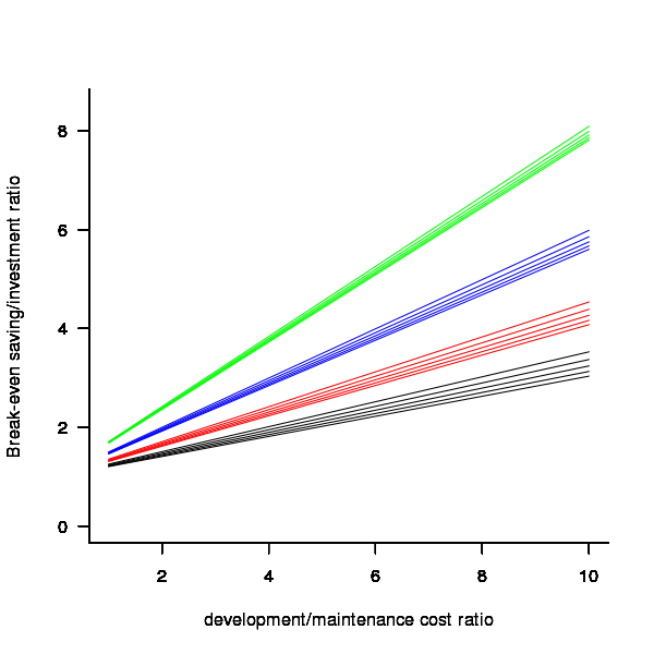
Figure 1. Break even saving/investment ratio for various system survival rates (black 0.9, red 0.8, blue 0.7 and green 0.6) and development/maintenance ratios; system lifetimes are 5.5, 6, 6.5, 7 and 7.5 years (ordered top to bottom)
Development and maintenance costs
Dunn’s PhD thesis <book Dunn_11> lists development and total maintenance costs (for the first five years) of 158 software systems from IBM. The systems varied in size from 34 to 44,070 man hours of development effort and from 21 to 78,121 man hours of maintenance.
The plot below shows the ratio of development to five year maintenance costs for the 158 software systems. The mean value is around one and if we assume equal spending during the maintenance period then  .
.
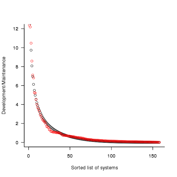
Figure 2. Ratio of development to five year maintenance costs for 158 IBM software systems sorted in size order. Data from Dunn <book Dunn_11>.
The best fitting common distribution for the maintenance/development ratio is the <Beta distribution>, a distribution often encountered in project planning.
Is there a correlation between development man hours and the maintenance/development ratio (e.g., do smaller systems tend to have a lower/higher ratio)? A Spearman rank correlation test between the maintenance/development ratio and development man hours gives:
|
showing very little connection between the two values.
Is the data believable?
While a single company dataset might be thought to be internally consistent in its measurement process, IBM is a very large company and it is possible that the measurement processes used were different.
The maintenance data applies to software systems that have not yet reached the end of their lifespan and is not broken down by year. Any estimate of total or yearly maintenance can only be based on assumptions or lifespan data from other studies.
System lifetime
A study by Tamai and Torimitsu <book Tamai_92> obtained data on the lifespan of 95 software systems. The plot below shows the number of systems surviving for at least a given number of years and a fit of an <Exponential distribution> to the data.
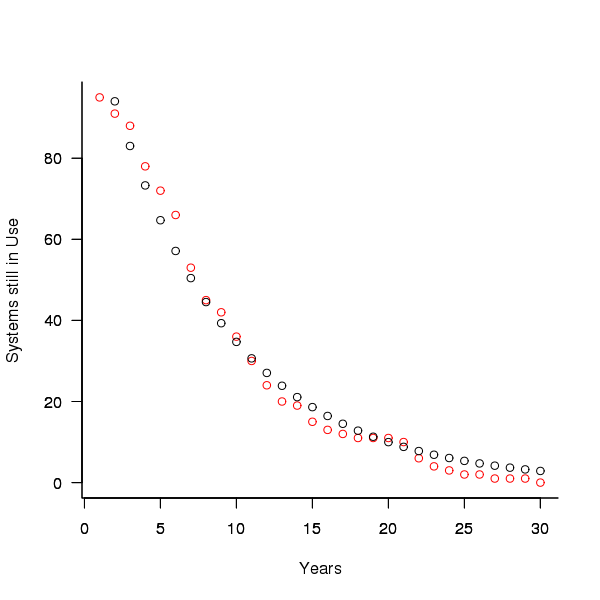
Figure 3. Number of software systems surviving to a given number of years (red) and an exponential fit (black, data from Tamai <book Tamai_92>).
The nls function gives  as the best fit, giving a half-life of 5.4 years (time for the number of systems to reduce by 50%), while rounding to
  gives a half-life of 6.6 years and reducing to
  a half life of 4.6 years.
It is worrying that such a small change to the estimated fit can have such a dramatic impact on estimated half-life, especially given the uncertainty in the applicability of the 20 year old data to today’s environment. However, the saving/investment ratio plot above shows that the final calculated value is not overly sensitive to number of years.
Is the data believable?
The data came from a questionnaire sent to the information systems division of corporations using mainframes in Japan during 1991.
It could be argued that things have stabilised over the last 20 years ago and complete software replacements are rare with most being updated over longer periods, or that growing customer demands is driving more frequent complete system replacement.
It could be argued that large companies have larger budgets than smaller companies and so have the ability to change more quickly, or that larger companies are intrinsically slower to change than smaller companies.
Given the age of the data and the application environment it came from a reasonably wide margin of uncertainty must be assigned to any usage patterns extracted.
Summary
Based on the available data an investment during development must recoup a benefit during maintenance that is at least twice as great in percentage terms to break even:
- systems with a yearly survival rate of less than 90% must have a benefit/investment rate greater than two if they are to break even,
- systems with a development/yearly maintenance rate of greater than 20% must have a benefit/investment rate greater than two if they are to break even.
The availanble software system replacement data is not reliable enough to suggest any more than that the estimated half-life might be between 4 and 8 years.
This analysis only considers systems that have been delivered and started to be used. Projects are cancelled before reaching this stage and including these in the analysis would increase the benefit/investment break even ratio.
Agreement between code readability ratings given by students
I have previously written about how we know nothing about code readability and questioned how the information content of expressions might be calculated. Buse and Weimer ran a very interesting experiment that asked subjects to rate short code snippets for readability (somebody please rerun this experiment using professional software developers).
I’m interested in measuring how well different students subjects agree with each other (I have briefly written about this before).
Short answer: Very little agreement between individual pairs, good agreement between rankings aggregated by year.
The longer answer is below as another draft section from my book Empirical software engineering with R book. As always comments welcome. R code and data here.
Readability
Source code is often said to have an attribute known as
A study by Buse and Weimer <book Buse_08> asked Computer Science students to rate short snippets of Java source code on a scale of 1 to 5. Buse and Weimer then searched for correlations between these ratings and various source code attributes they obtained by measuring the snippets.
Humans hold diverse opinions, have fragmented knowledge and beliefs about many topics and vary in their cognitive abilities. Any study involving human evaluation that uses an open ended problem on which subjects have had little experience is likely to see a wide range of responses.
Readability is a very nebulous term and students are unlikely to have had much experience working with source code. A wide range of responses is to be expected and the analysis performed here aims to check the degree of readability rating agreement between the subjects.
Data
The data made available by Buse and Weimer are the ratings, on a scale of 1 to 5, given by 121 students to 100 snippets of source code. The student subjects were drawn from those taking first, second and third/fourth year Computer Science degree courses and postgraduates at the researchers’ University (17, 65, 31 and 8 subjects respectively).
The postgraduate data was not used in this analysis because of the small number of subjects.
The source of the code snippets is also available but not used in this analysis.
Is the data believable?
The subjects were not given any instructions on how to rate the code snippets for readability. Also we don’t know what outcome they were trying to achieve when rating, e.g., where they rating on the basis of how readable they personally found the snippets to be, or rating on the basis of the answer they would expect to give if they were being tested in an exam.
The subjects were students who are learning about software development and many of them are unlikely to have had any significant development experience outside of the teaching environment. Experience shows that students vary significantly in their ability to read and write source code and a non-trivial percentage do not go on to become software developers.
Because the subjects are at an early stage of learning about code it is to be expected that their opinions about readability will change while they are rating the 100 snippets. The study did not include multiple copies of some snippets, this would have enabled the consistency of individual subject responses to be estimated.
The results of many studies <book Annett_02> has shown that most subject ratings are based on an ordinal scale (i.e., there is no fixed relationship between the difference between a rating of 2 and 3 and a rating of 3 and 4), that some subjects are be overly generous or miserly in their rating and that without strict rating guidelines different subjects apply different criteria when making their judgements (which can result a subject providing a list of ratings that is inconsistent with every other subject).
Readability is one of those terms that developers use without having much idea what they and others are really referring to. The data from this study can at most be regarded as treating readability to be whatever each subject judges it to be.
Predictions made in advance
Is the readability rating given to code snippets consistent between different students on a computer science course?
The hypothesis is that the between student consistency of the readability rating given to code snippets improves as students progress through the years of attending computer science courses.
Applicable techniques
There are a variety of techniques for estimating rater agreement. <Krippendorff’s alpha> can be applied to ordinal ratings given by two or more raters and is used here.
Subjects do not have to give the same rating to share some degree of consistent response. Two subjects may share a similar pattern of increasing/decreasing/stay the same ratings across snippets. The <Spearman rank correlation> coefficient can be used to measure the correlation between the rank (i.e., relative value within sequence) of two sequences.
Results
When creating the snippets the researchers had no method of estimating what rating subjects would give to them and so there is no reason to expect a uniform distribution of rating values or any other kind of distribution of rating values.
The figure below is a boxplot of the rating of the first 50 code snippets rated by second year students and suggests that many subject ratings are within ±1 of each other.
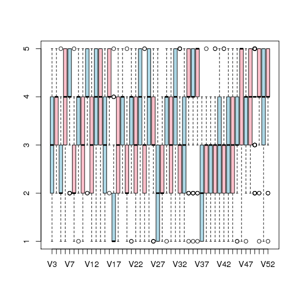
Figure 1. Boxplot of ratings given to snippets 1 to 50 by second year students (colors used to help distinguish boxplots for each snippet).
Between subject rating agreement
The Krippendorff alpha and mean Spearman rank correlation coefficient (the coefficient is calculated for every pair of subjects and the mean value taken) was obtained using the kripp.alpha and meanrho functions from the irr package (a <Jackknife> was used to obtain the following 95% confidence bounds):
Krippendorff's alpha cs1: 0.1225897 0.1483692 cs2: 0.2768906 0.2865904 cs4: 0.3245399 0.3405599 mean Spearman's rho cs1: 0.1844359 0.2167592 cs2: 0.3305273 0.3406769 cs4: 0.3651752 0.3813630 |
Taken as a whole there is a little of agreement. Perhaps there is greater consensus on the readability rating for a subset of the snippets. Recalculating using only using those snippets whose rated readability across all subjects, by year, has a standard deviation less than 1 (around 22, 51 and 62% of snippets respectively) shows some improvement in agreement:
Krippendorff's alpha cs1: 0.2139179 0.2493418 cs2: 0.3706919 0.3826060 cs4: 0.4386240 0.4542783 mean Spearman's rho cs1: 0.3033275 0.3485862 cs2: 0.4312944 0.4443740 cs4: 0.4868830 0.5034737 |
Between years comparison of ratings
The ratings from individual subjects is only available for one of their years at University. Aggregating the answers from all subjects in each year is one method of obtaining readability information that can be used to compare the opinions of students in different years.
How can subject ratings be aggregated to rank the 100 code snippets in order of what a combined group consider to be readability? The relatively large variation in mean value of the snippet ratings across subjects would result in wide confidence bounds for an aggregate based on ratings. Mapping each subject’s rating to a ranking removes the uncertainty caused by differences in mean subject ratings.
With 100 snippets assigned a rating between 1 and 5 by each subject there are going to be a lot of tied rankings. If, say, a subject gave 10 snippets a rating of 5 the procedure used is to assign them all the rank that is the mean of the ranks the 10 of them would have occupied if their ratings had been very slightly different, i.e., (1+2+3+4+5+6+7+8+9+10)/10 = 5.5. This process maps each students readability ratings to readability rankings, the next step is to aggregate these individual rankings.
The R_package[RankAggreg] package contains a variety of functions for aggregating a collection rankings to obtain a group ranking. However, these functions use the relative order of items in a vector to denote rank, and this form of data representations prevents them supporting ranked lists containing items having the same rank.
For this analysis a simple aggregate ranking algorithm using Borda’s method <book lin_10> was implemented. Borda’s method for creating an aggregate ranking operates on one item at a time, combining all of the subject ranks for that item into a single rank. Methods for combining ranks include taking their mean, their geometric mean and the square-root of the sum of their squares; the mean value was used for this analysis.
An aggregate ranking was created for subjects in years one, two and four and the plot below compares the ranking between 1st/2nd year students (left) and 2nd/4th year students (right). The order of the second year student snippet rankings have been sorted and the other year rankings for the snippets mapped to the corresponding position.
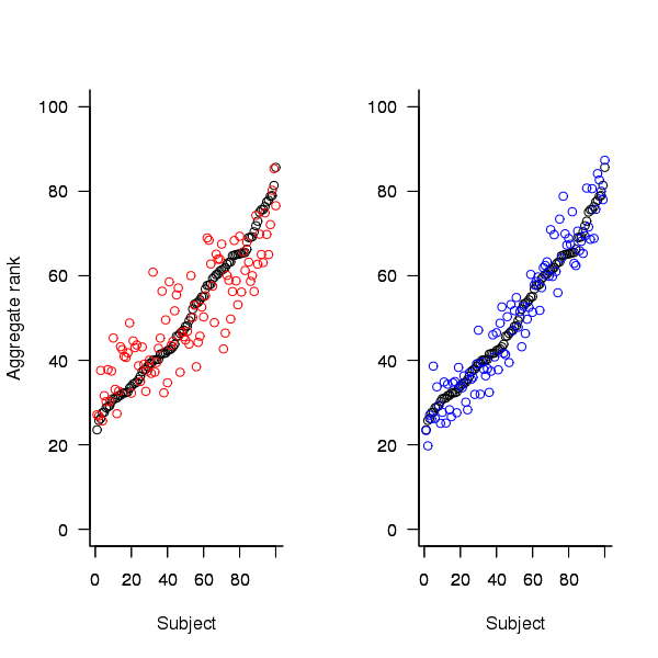
Figure 2. Aggregated ranking of snippets by subjects in years 1 and 2 (red and black) and years 2 and 4 (black and blue). Snippets have been sorted by year 2 ranking.
The above plot seems to show that at the aggregated year level there is much greater agreement between the 2nd/4th years than any other year pairing and measuring the correlation between each of the years using <Kendall’s tau>:
cs1.tau cs2.tau cs3.tau 0.6627602 0.6337914 0.8199636 |
confirms the greater agreement between this aggregate year pair.
Individual subject correlation to year aggregate ranking
To what extend to subject ratings correlate with their corresponding year aggregate? The following plot gives the correlation, using Kendall’s tau, between each subject and their corresponding year aggregate ranking.
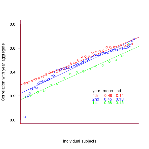
Figure 3. Correlation, using Kendall’s tau, between each subject and their corresponding year aggregate ranking.
The least squares fit shows that the variation in correlation across subjects in any year is very similar (removal of outliers in year 2 would make the lines almost parallel); the mean again shows a correlation that increases with year.
Discussion
The extent to which this study’s calculated values of rater agreement and correlation are considered worthy of further attention depends on the use to which the results will be put.
- From the perspective of trained raters the subject agreement in this study is very low and the rating have no further use.
- From the research perspective the results show that the concept of readability in the computer science student population has some non-zero substance to it that might be worth further study.
- From an overall perspective this study provides empirical evidence for a general lack of consensus on what constitutes readability.
It is not surprising that there is little agreement between student subjects on their readability rating, they are unlikely to have had much experience reading code and have not had any training in rating code for readability.
Professional developers will have spent years working with code and this experience is likely to have resulted in the creation of stable opinions on code readability. While developers usually work with code that is much longer than the few lines contained in the snippets used by Buse and Weimer, this experiment format is easy to administer and supports a fine level of control, i.e., allows a small set of source attributes of interest to be presented while excluding those not of interest. Repeating this study using such people as subjects would show whether this experience results in convergence to general agreement on the readability rating of code.
Summary of findings
The agreement between students readability ratings, for short snippets of code, improves as the students progress through course years 1 to 4 of a computer science degree.
While there is very good aggregated group agreement on the relative ranking of the readability of code snippets there is very little agreement between pairs of individuals.
- Two students chosen at random from within a year will have a low Spearman rank correlation coefficient for their rating of code snippet readability.
- Taken as a yearly aggregate there is a high degree of agreement between years two and four and less, but still good agreement between year 1 and other years.
- There is a broad range of correlations, from poor to good, between year aggregates and student subjects in the corresponding year.
Sequence generation with no duplicate pairs
Given a fixed set of items (say, 6 A, 12 B and 12 C) what algorithm will generate a randomised sequence containing all of these items with any adjacent pairs being different, e.g., no AA, BB or CC in the sequence? The answer would seem to be provided in my last post. However, turning this bit of theory into practice uncovered a few problems.
Before analyzing the transition matrix approach let’s look at some of the simpler methods that people might use. The most obvious method that springs to mind is to calculate the expected percentage of each item and randomly draw unused items based on these individual item percentages, if the drawn item matches the current end of sequence it is returned to the pool and another random draw is made. The following is an implementation in R:
seq_gen_rand_total=function(item_count) { last_item=0 rand_seq=NULL # Calculate each item's probability item_total=sum(item_count) item_prob=cumsum(item_count)/item_total while (sum(item_count) > 0) { # To recalculate on each iteration move the above two lines here. r_n=runif(1, 0, 1) new_item=which(r_n < item_prob)[1] # select an item if (new_item != last_item) # different from last item? { if (item_count[new_item] > 0) # are there any of these items left? { rand_seq=c(rand_seq, new_item) last_item=new_item item_count[new_item]=item_count[new_item]-1 } } else # Have we reached a state where a duplicate will always be generated? if ((length(which(item_count != 0)) == 1) & (which(item_count != 0)[1] == last_item)) return(0) } return(rand_seq) } |
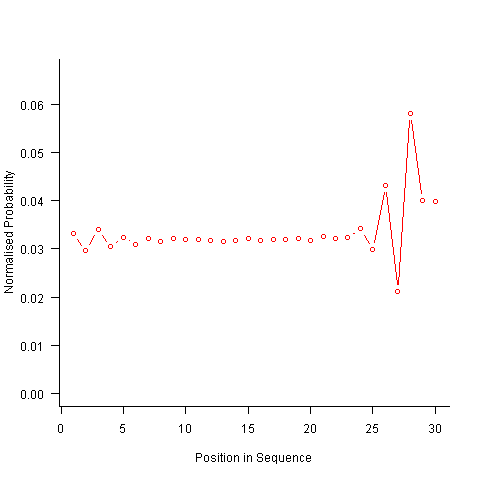
For instance, with 6 A, 12 B and 12 C, the expected probability is 0.2 for A, 0.4 for B and 0.4 for C. In practice if the last item drawn was a C then only an A or B can be selected and the effective probability of A is effectively increased to 0.3333. The red circles in the figure below show the normalised probability of an A appearing at different positions in the sequence of 30 items (averaged over 200,000 random sequences); ideally the normalised probability is 0.0333 for all positions in the sequence In practice the first position has the expected probability (there is no prior item to disturb the probability), the probability then jumps to a higher value and stays sort-of the same until the above-average usage cannot be sustained any more and there is a rapid decline (the sudden peak at position 29 is an end-of-sequence effect I talk about below).
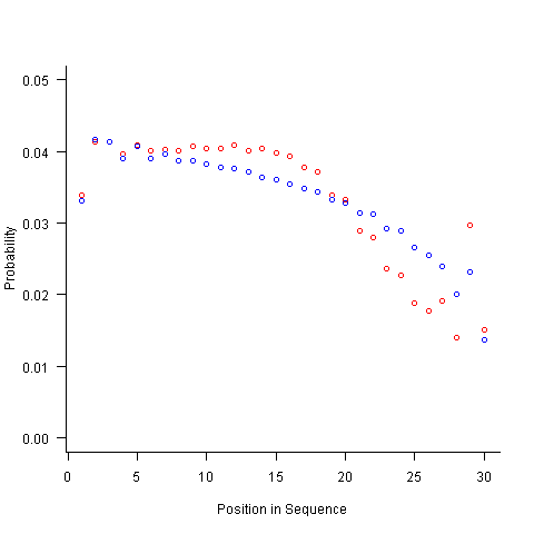
What might be done to get closer to the ideal behavior? A moments thought leads to the understanding that item probabilities change as the sequence is generated; perhaps recalculating item probabilities after each item is generated will improve things. In practice (see blue dots above) the first few items in the sequence have the same probabilities (the slight differences are due to the standard error in the samples) and then there is a sort-of consistent gradual decline driven by the initial above average usage (and some end-of-sequence effects again).
Any sequential generation approach based on random selection runs the risk of reaching a state where a duplicate has to be generated because only one kind of item remains unused (around 80% and 40% respectively for the above algorithms). If the transition matrix is calculated on every iteration it is possible to detect the case when a given item must be generated to prevent being left with unusable items later on. The case that needs to be checked for is when the percentage of one item is greater than 50% of the total available items, when this occurs that item must be generated next, e.g., given (1 A, 1 B, 3 C) a C must be generated if the final list is to have the no-pair property.
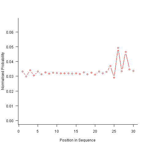
Now the transition matrix approach. Here the last item generated selects the matrix row and a randomly generated value selects the item within the row. Let’s start by generating the matrix once and always using it to select the next item; the resulting normalised probability stays constant for much longer because the probabilities in the transition matrix are not so high that items get used up early in the sequence. There is a small decline near the end and the end-of-sequence effects kick in sooner. Around 55% of generated sequences failed because two of the items were used up early leaving a sequence of duplicates of the remaining item at the end.
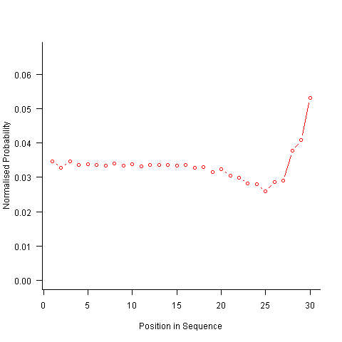
Finally, or so I thought, the sought after algorithm using a transition matrix that is recalculated after every item is generated. Where did that oscillation towards the end of the sequence come from?
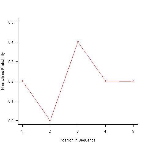
After a some head scratching I realised that the French & Perruchet algorithm is based on redistribution of the expected number of items pairs. Towards the end of the sequence there is a growing probability that the number of remaining As will have dropped to one; it is not possible to create an AA pair from only one A and the assumptions behind the transition matrix calculation break down. A good example of the consequences of this breakdown is the probability distribution for the five item sequences that the algorithm might generate from (1 A, 2 B, 2 C); an A will never appear in position 2 of the sequence:
After various false starts I decided to update the French & Perruchet algorithm to include and end-of-sequence state. This enabled me to adjust the average normalised probability of the main sequence (it has be just right to avoid excess/missing probability inflections at the end), but it did not help much with the oscillations in the last five items (it has to be said that my updated calculations involve a few hand-waving approximations of their own).
I found that a simple, ad hoc solution to damp down the oscillations is to increase any single item counts to somewhere around 1.3 to 1.4. More thought is needed here.
Are there other ways of generating sequences with the desired properties? French & Perruchet give one in their paper; this generates a random sequence, removes one item from any repeating pairs and then uses a random insert and shuffle algorithm to add back the removed items. Robert French responded very promptly to my queries about end-of-sequence effects, sending me a Matlab program implementing an updated version of the algorithm described in the original paper that he tells does not have this problem.
The advantage of the transition matrix approach is that the next item in the sequence can be generated on an as needed basis (provided the matrix is calculated on every iteration it is guaranteed to return a valid sequence if one exists; of course this recalculation removes some randomness for the sequence because what has gone before has some influence of the item distribution that follows). R code used for the above analysis.
I have not been able to locate any articles describing algorithms for generating sequences that are duplicate pair free and would be very interested to hear of any reader experiences.
Recent Comments