The Shape of Code

At the technical level the Oracle ‘Java’ lawsuit against Google is not really about Java at all. The patents cited in the lawsuit (5,966,702, 6,061,520, 6,125,447, 6,192,476, RE38,104, 6,910,205 and 7,426,720) involve a variety of techniques that might be used in the implementation of a virtual machine supporting JIT compilation for software written in any language; Oracle does not get into the specifics of which parts of Android make use of these patented techniques (Google has not released the Dalvik source code). With regard to the claimed copyright infringement, I have no idea what Oracle claim has been copied; as I understand it Android uses Apache’s Harmony code for its Dalvik VM runtime library, but there is a possibility that it might have used some of Oracle’s gpl’ed code.

No doubt Google’s lawyers will be asking for specific details and once these are provided they have three options: 1) find prior art that invalidates the patent, 2) recode the implementation so it does not infringe the patent or 3) negotiate a license with Oracle.

My only experience in searching for prior art was as an adviser to the Monitoring Trustee appointed by the European Commission in the EU/Microsoft competition court case; Microsoft’s existing patents were handled by a patent lawyer and I looked at some of the non-patented innovations being claimed by Microsoft.

The obvious tool to use in a search for prior art is Google and this worked well for me provided the information was created after the mid to late 1990s. The cut-off date for historical searches seemed to be around 1993 (this all happened before Google Books was released). Other sources of information included old books (I had not moved in 15 years and my book collection had not been culled), computer manuals and one advisor found what he was looking for in some old computer magazines bought on e-bay.

Some claimed innovations appeared so blindingly obvious that it was difficult to believe that anybody would bother mentioning it in a print. Oracle’s patent 6,910,205
“Interpreting functions utilizing a hybrid of virtual and native machine instructions” (actually a continuation of 6,513,156, filed five years earlier in 1997) describes an obvious method of handling the interface between interpreted and JIT compiled code.

My only implementation experience in this area does predate the Oracle patent (I wrote a native code generator for the UCSD Pascal p-code machine in the mid-80s) but the translation occurred before program execution and so is not appropriate prior art. Virtual machines fell out of favor in the late 80s and when they were revived by Java 10 years later I was no longer working on compilers

Fans of Lisp are always claiming that everything was first done by the Lisp community and there were certainly Lisp compilers around in the 1980s, but I’m not sure if any of them worked during program execution.

Of course Groklaw have started following this case. Kodak has shown that it is possible to win in court over Java related patents. The SunOracle/Microsoft Java lawsuit in the late 1990s was a contract dispute and not about patents/copyright, but still about money/control.

I’m not aware of any previous language implementation patent lawsuits that have gone to court. It will be interesting to see how much success Google have in finding prior art and whether it is possible to implement a JVM that does not make use of any of the techniques specified in the Oracle patents (I suspect that they have a few more that they have not yet cited).

People look for patterns and expect others to follow patterns of behavior. Some preliminary data from a game of Colonel Blotto run by a group of Cornell University graduate students provides a vivid example of the existence of these behavior patterns.

In the Cornell implementation of the Colonel Blotto game, there are 10 fields and 100 soldiers. A player specifies how many soldiers are posted to each of the 10 fields. Players don’t know what the opposing players will do. In each field the battle is decided by whoever has the most soldiers with equal numbers resulting in a draw. Whoever wins the most battles wins the war.

One possible soldiers per field sequence is 10 10 10 10 10 10 10 10 10 10 and another is 1 11 11 11 11 11 11 11 11 11. The second sequence will lose in the first field, but win the other 9, and therefore win the war. A third sequence is 9 11 12 12 12 12 8 8 8 8 which beats the second sequence but only draws against the first.

The number of ways of placing indistinguishable soldiers into fields is:

The following original analysis assumes that the soldiers are distinguishable, which they are not and so the number calculated is way too large (thanks to Forbes at The Virtuosi for pointing this out): There are 10 ways of placing the first soldier, 10 ways of placing the second and so on, giving possible arrangements.

Some arrangements obviously always lose (25 25 25 25 0 0 0 0 0 0) and won’t be played; it seems reasonable to assume that no field will contain zero (I will talk about putting 0 in one field later), so having a field contain 1 is a draw at best. Lets assume that all fields contain at least 2 soldiers, which means we have 80 left to arrange giving possibilities; a very big drop in possibilities but still a huge number.

The more soldiers appearing in a field the more likely a win will occur there, but after a while the law of diminishing returns kicks in and losses occurring in understaffed fields will be greater. Lets assume that people decide never to put more than 20 soldiers in a field; how many possibilities does this rule out? If one field initially contains 21 soldiers and the others 2 each the remaining 61 soldiers create unused possibilities, putting 21 soldiers in the second field generates a bit less than new possibilities; lets round up and say there are a total of unused possibilities. Compared to the unused is small enough to be ignored.

is such a big number that Chimpanzees randomly typing away since the dawn of time are unlikely to create any discernible pattern in the landscape.

If the players in this game had given random answers what would be the mean number of points scores and its variance?

Comparing the soldier sequence given by player A against the sequence given by player B produces 11 possible scores, {0, 10}, {1, 9} … {5, 5} … {10, 0}, five of them resulting in a win for A, five in a win for B and one in a draw. With 2 points for a win, 1 point for a draw and 0 points for a loss the expected number of points for each of the two players is 1, so for players the expected mean of each player is . In a game containing 550 players (the number that had played when I extracted the score results today; 347 had played in the preliminary Cornell data set) we would expect the average score to be 550.

The variance can be calculated from:

The standard deviation about our mean is or 22.4.

Plotting a histogram of points scored, at the time of writing, we get the following:

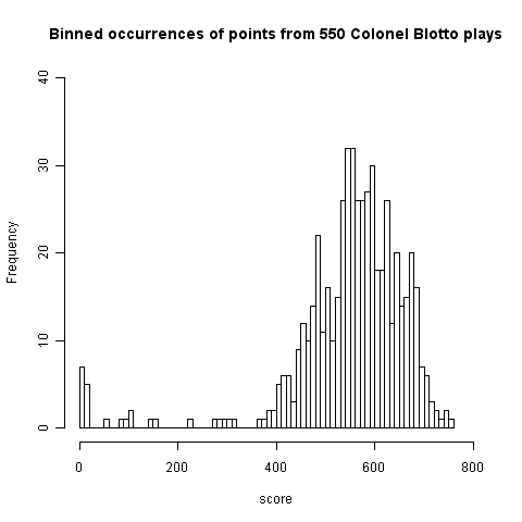
This has a peak at 550 where we would expect it and its width is two standard deviations However those ‘side-lobes’ were not expected and they are asymmetric. I think the reason for these unexpected ‘side-lobes’ is that some players give multiple answers, attempting to improve their ranking (some strategy name are suggestive of retries with modified strategies) and consequently decreasing the total points of other players. A search space of sequences is so large that we would not expect players to be able to learn from the results of previously submitted sequences unless many of the previously submitted sequences followed some pattern that they could recognise.

What pattern of behavior might players follow? I can imagine players starting low/high and then shifting to high/low, perhaps following this sequence two or more times.

A preliminary summary of some of the data seen so far by Alex Alemi gave me enough information to figure out a sequence, in three attempts, that ranked 1st (a typo on my part prevented it being on the second attempt); my sequence of player names is averages, aver_p6, low_high_dip, followed by a bit of tuning: low_high_dipish, lohilohi_slide, followed by two experiments: the_well, heat_map, and user fooly started getting close and I tuned the sequence a bit more lohilohi_sliiide.

I used the sequences from the top 25 ranked players for my analysis and did not make any attempt to deduce other player patterns. My first attempt averaged the number of soldiers in each field, ranked 62nd as I write (aver_p6). Then I spotted that several distribution patterns existed, I picked what looked like the most promising and averaged over it (by eye) to get the then current to number 1 (currently languishing in 8th).

Had I put a bit more thought into things I could also have used the heat map near the bottom of the post (thanks to Alex Alemi for letting me post a copy here; “With Y soldiers in slot X, what percentage of the existing strategies do you beat in slot X.”):

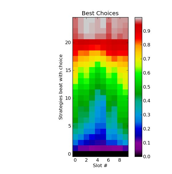
This shows one pattern (in light blue) where players are following the pattern low-high-low-high-low with the second low being very precipitous. The patterns visible in green are more complicated, but still contain a recurring low-high theme.

I know next to nothing about autocorrelation and so do not have any bright ideas about how to use of this data to improve my score. The heat_map sequence (7 8 9 12 15 16 9 11 7 6) attempts to follow the light blue pattern and is ranked 296 as I write, just under half way down the rankings and something to be expected from following an average.

Once a major pattern has been deduced ‘extra’ soldiers will be needed to outnumber the other players most of the time. One option is to be willing to always lose in one field (e.g., the one usually requiring the most soldiers) and use the freed up resources to win elsewhere. I have only made one attempt using this strategy (the_well: 5 6 7 11 19 0 14 20 13 5, ranked 72 as I write).

It is possible that common patterns of behavior are created through reinforcement. Early players create an initial configuration of results and slightly later players attempt to find it, perhaps visualizing a pattern where none actually exists. If enough people follow the same trail they will create the pattern that others can will try to follow. Results from other Colonel Blotto games exhibit a pattern of behavior that is different from the one in the Cornell dataset (I have only seen what is publicly available)

Many coding guidelines recommend against the presence of unreachable code in source; the argument being that while the code itself is harmless its presence suggests something has gone wrong somewhere else. As a member of the MISRA C++ coding guidelines committee I unsuccessfully argued against this recommendation being included on the grounds of lack of evidence that unreachable code was a significantly strong indicator of a fault and the complications caused by wanting allow certain kinds of what appeared to be unreachable code (e.g., that used by defensive programming practices).

I was recently reading the PhD thesis of Yichen Xie and found some very interesting analysis of correlation between various kinds of dead code (redundant code was one of the kinds) and faults.

Yichen Xie took a course grained approach to finding a correlation between redundant code and faults. He simply counted the numbers of files that did/did not contain redundant code and the number of corresponding files known to contain what he called a hard bug. The counts were as follows (statistical analysis using the contingency table method gives a probability of well below 0.01 for these values being generated by the null hypothesis):

               Hard Bugs
Dead Code     Yes     No   Totals
  Yes         133     135    268
   No         418    1369   1787
Totals        551    1504   2055

These counts show that if one of the 2,055 files was picked at random the expectation of it containing a Hard Bug is 27%, for one of the files containing unreachable code the expectation is 50% and for files not containing unreachable code it is 23%. So picking a file containing unreachable code almost doubles the expectation of a Hard Bug being found in that file.

These measurements do not attempt to make a connection between the unreachable code contained in a file and any fault contained within that file. How would the counts change if they were based on their being some form of logical connection between the redundant code and the fault? The counts suggest at least a 50% false positive rate, but then faults that generate unreachable code may be the result of high level semantic issues that are less likely to be detected by a casual reading of the source or by static analysis tools.

The hoped for consequence of a coding guideline requiring the removal of unreachable code is that developers analyze the code to understand why the code is unreachable and that in many cases this will result in a fault being uncovered and fixed; the worst case scenario is that they simply delete the unreachable code.

This research has caused me to upgrade the significance I give to unreachable code but I remain unconvinced that the false positive rate is sufficiently low for it to be a worthwhile coding guideline.